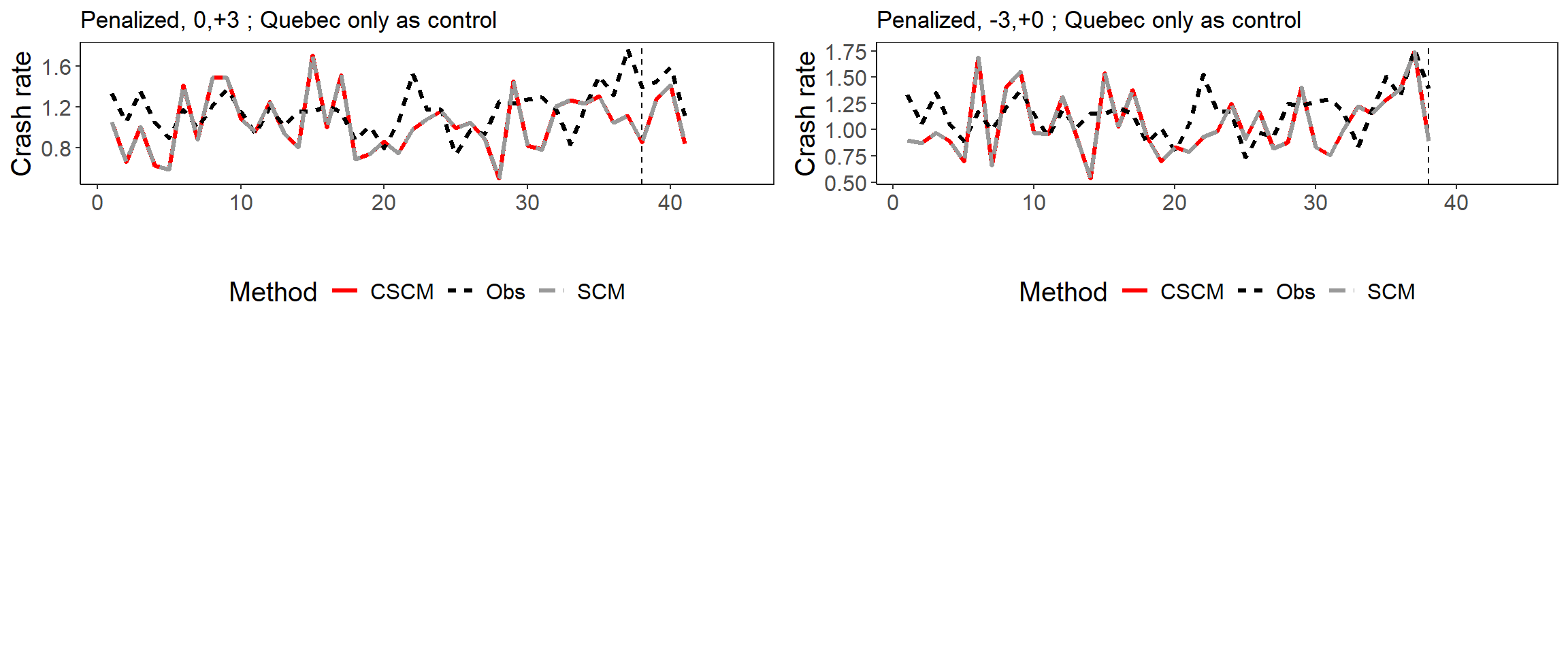
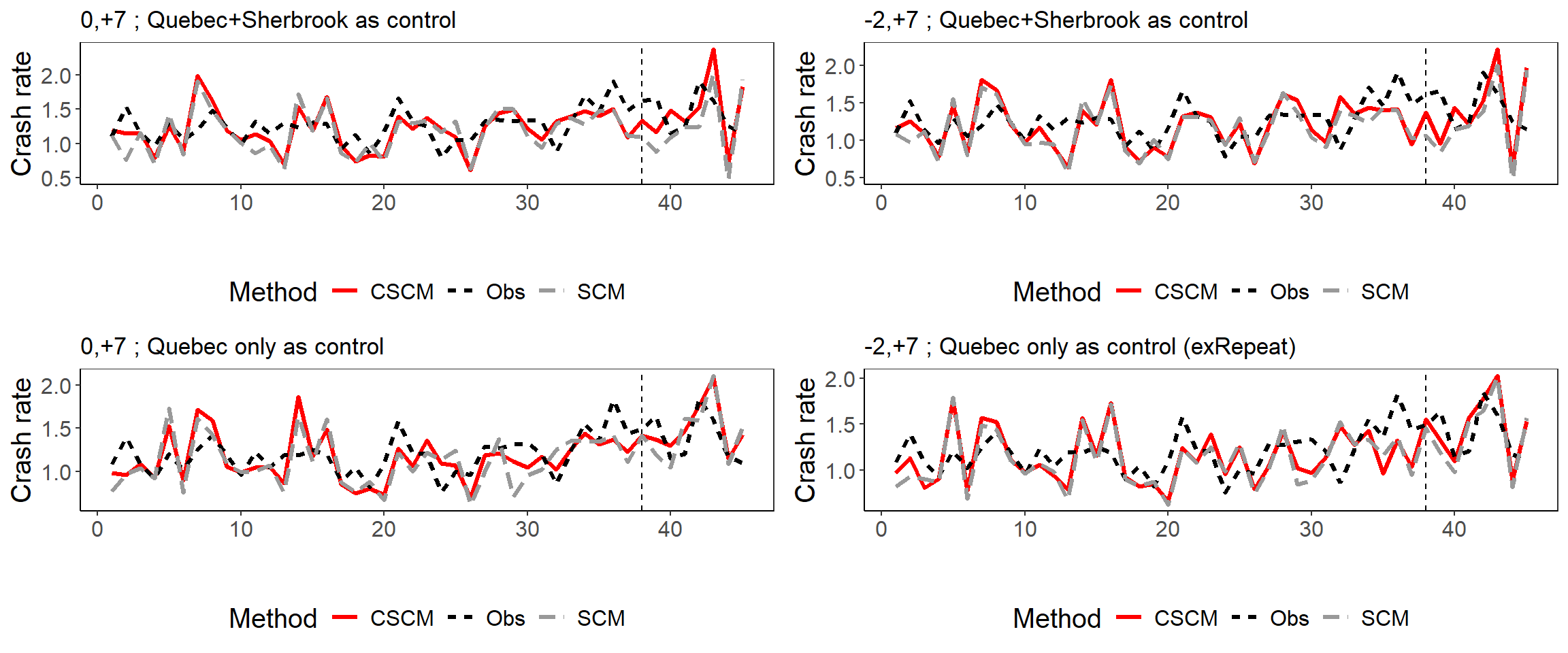
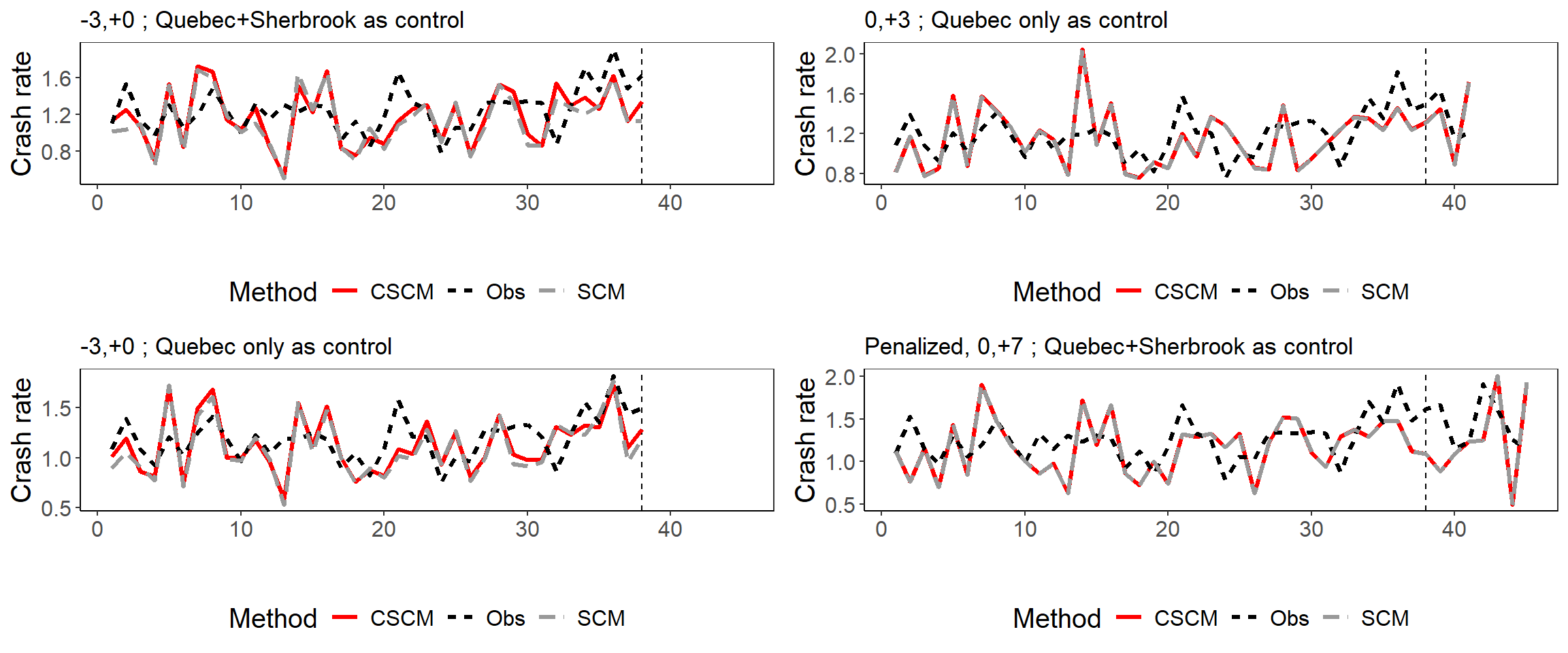
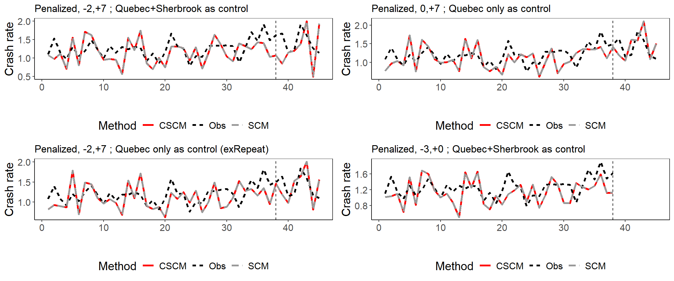
── Conflicts ────────────────────────────────────────── tidyverse_conflicts() ──
✖ dplyr::filter() masks stats::filter()
✖ dplyr::lag()    masks stats::lag()
ℹ Use the conflicted package (<http://conflicted.r-lib.org/>) to force all conflicts to become errors

Adjuntando el paquete: 'dagitty'


The following object is masked from 'package:rio':

    convert


Adjuntando el paquete: 'ggdag'


The following object is masked from 'package:stats':

    filter


Adjuntando el paquete: 'kableExtra'


The following object is masked from 'package:dplyr':

    group_rows


Cargando paquete requerido: Matrix


Adjuntando el paquete: 'Matrix'


The following objects are masked from 'package:tidyr':

    expand, pack, unpack


Adjuntando el paquete: 'lme4'


The following object is masked from 'package:rio':

    factorize


This is DHARMa 0.4.7. For overview type '?DHARMa'. For recent changes, type news(package = 'DHARMa')

Cargando paquete requerido: carData


Adjuntando el paquete: 'car'


The following object is masked from 'package:purrr':

    some


The following object is masked from 'package:dplyr':

    recode


Cargando paquete requerido: Rcpp

Loading 'brms' package (version 2.22.0). Useful instructions
can be found by typing help('brms'). A more detailed introduction
to the package is available through vignette('brms_overview').


Adjuntando el paquete: 'brms'


The following object is masked from 'package:glmmTMB':

    lognormal


The following object is masked from 'package:lme4':

    ngrps


The following object is masked from 'package:stats':

    ar


This is bayesplot version 1.12.0

- Online documentation and vignettes at mc-stan.org/bayesplot

- bayesplot theme set to bayesplot::theme_default()

   * Does _not_ affect other ggplot2 plots

   * See ?bayesplot_theme_set for details on theme setting


Adjuntando el paquete: 'bayesplot'


The following object is masked from 'package:brms':

    rhat


This is loo version 2.8.0

- Online documentation and vignettes at mc-stan.org/loo

- As of v2.0.0 loo defaults to 1 core but we recommend using as many as possible. Use the 'cores' argument or set options(mc.cores = NUM_CORES) for an entire session.

- Windows 10 users: loo may be very slow if 'mc.cores' is set in your .Rprofile file (see https://github.com/stan-dev/loo/issues/94).

##
## Synth Package: Implements Synthetic Control Methods.


## See https://web.stanford.edu/~jhain/synthpage.html for additional information.


Welcome to emmeans.
Caution: You lose important information if you filter this package's results.
See '? untidy'

Registered S3 method overwritten by 'lfe':
  method    from
  nobs.felm broom


Adjuntando el paquete: 'plm'


The following objects are masked from 'package:dplyr':

    between, lag, lead


Registered S3 method overwritten by 'quantmod':
  method            from
  as.zoo.data.frame zoo


Adjuntando el paquete: 'forecast'


The following object is masked from 'package:brms':

    ma


Adjuntando el paquete: 'cowplot'


The following object is masked from 'package:lubridate':

    stamp


Cargando paquete requerido: stats4


Adjuntando el paquete: 'bbmle'


The following object is masked from 'package:brms':

    parnames


The following object is masked from 'package:dplyr':

    slice
Code
#special repository indicated or the packageif(!require(weathercan)){install.packages("weathercan", repos =c("https://ropensci.r-universe.dev", "https://cloud.r-project.org")); library(weathercan) }
Cargando paquete requerido: weathercan
Warning: package 'weathercan' was built under R version 4.4.3
As of v0.7.2, the `normals` column in `stations()` reflects whether or not there
are *any* normals available (not just the most recent).
#-- Fórmula 1 – ventana de riesgo#-- Accidentes por exceso de velocidad#--Weather (temperatura, lluvia…)#-- Day-of-week / season / calendario#-- Rasgos fijos de la comuna (infraestructura, cultura vial)dag <-dagitty('dag { F1 [exposure, pos="-2.000, 0.000"] Y [outcome, pos=" 2.000, 0.000"] W [adjusted, pos="-1.000, 3.250"] DOW [adjusted, pos="-1.000, -3.250"] U [unobserved, pos=" -3.000, 2.000"] F1 -> Y W -> F1 W -> Y DOW -> F1 DOW -> Y U -> Y}')# coords <- data.frame(# x = c(-2, 2, -1, -1, 3), # ← exactly the positions you want# y = c( 0, 0, 3, -3, 0),# row.names = c("F1", "Y", "W", "DOW", "U")# )# # coordinates(dag) <- coords # fix positions inside dagitty# datatidy <-tidy_dagitty(dag)edges <- tidy %>%# sólo flechas →filter(direction =="->") %>%mutate(edge_colour =if_else(name =="U", "grey60", "black"),edge_linetype =if_else(name =="U", "dashed", "solid"),edge_linewidth =0.9# grosor )nodes <- tidy %>%data.frame() |>distinct(name, x, y) %>%# nodosmutate(shape =if_else(name %in%c("W","DOW"),"square", "circle"))## 3 · Plot -------------------------------------------------------------ggplot() +geom_dag_edges_link( # ← solo flechas →data = edges,aes(x = x, y = y, xend = xend, yend = yend,edge_colour = edge_colour,edge_linetype = edge_linetype,edge_linewidth = edge_linewidth) ) +geom_dag_node(data = nodes,aes(x = x, y = y, shape = shape),fill ="white", colour ="black", size =18 ) +geom_dag_text(data = nodes, aes(x = x, y = y, label = name)) +scale_shape_manual(values =c(square =15, circle =16)) +#scale_edge_colour_identity() +#scale_edge_linetype_identity() +#edge_width_identity() + # usa edge_width_identity() si tu ggraph ≤ 2.0theme_void()+theme(legend.position ="none")
Code
library(DHARMa)#simulationOutput <- simulateResiduals(fittedModel = model_did1, plot = TRUE)cities <-unique(collisions_weather_corr$cluster)for (c in cities) {cat("\nEvaluando autocorrelación para cluster:", c, "\n") city_data <- collisions_weather_corr %>%filter(cluster == c) %>%arrange(iso_yday) indices <-which(collisions_weather_corr$cluster == c) city_residuals <- simulationOutput$scaledResiduals[indices]# Verificar que city_data y city_residuals tengan la misma longitudif(length(city_residuals) !=nrow(city_data)) {cat("Error: longitud de residuos y datos no coincide para cluster:", c, "\n")next }# Verificar que no haya NA en residuos ni en fechasif(any(is.na(city_residuals)) ||any(is.na(city_data$date))) {cat("Error: NA en residuos o fechas para cluster:", c, "\n")next }# Ordenar residuos según fechas order_idx <-order(city_data$iso_yday) city_data <- city_data[order_idx, ] city_residuals <- city_residuals[order_idx]print(paste("Length residuos:", length(city_residuals)))print(paste("Length fechas:", length(city_data$date)))print(paste("Duplicados fechas:", any(duplicated(city_data$date))))print(paste("NA en residuos:", sum(is.na(city_residuals))))# Verificar que fechas estén ordenadas y sin duplicadosif(any(duplicated(city_data$date))) {cat("Error: fechas duplicadas para cluster:", c, "\n")next }# Finalmente, llamar a la funcióntryCatch({testTemporalAutocorrelation(city_residuals, time = city_data$date)mtext(text =paste("Autocorr, cluster:", c), side =3, line =3, cex =1.2, font =2) }, error =function(e) {cat("Error en testTemporalAutocorrelation para cluster:", c, "\n", e$message, "\n") })}invisible("No hay evidencia significativa de autocorrelación temporal en los residuos del modelo para ninguna de las ciudades.")# simulationOutput <- simulateResiduals(fittedModel = model_final, plot = TRUE)# testDispersion(simulationOutput)# testZeroInflation(simulationOutput)
GNM
Code
# Case-crossover design# # Methods:# Only cases: cardiovascular defects 3870# # Exposure:# Case window: trimethoprim use any time during the second# and third months after the last menstrual period,# Reference window: use in 2 months prior to last menstrual# period within mothers of case infants.# Secondary reference windows: and 2 months prior and 2# months after the primary reference window# # Analysis:# #https://docs.google.com/document/d/1shhxi_PEkgc8N4riqV4lOowPcGPo2mdj4-PGA779oUk/edit?tab=t.0#https://drive.google.com/drive/u/0/folders/1gwdKKOVZd2JEHmb0oXt34FSpvea1oH7G no aplica tanto potque el análisis es por persona, es Conditional logistic regression y ve mortalidad. se busca para esa misma persona variables como días de tiempo#https://docs.google.com/presentation/d/1Khvb5C8ZTaw3HKfvx3oAKD7fBZHPcd_v/edit?slide=id.p42#slide=id.p42#https://docs.google.com/spreadsheets/d/1znDbWVXO2A5uSKiVazQwFJKZcrrH-VZXnQsG-INBQ-w/edit?gid=0#gid=0#https://drive.google.com/drive/u/0/folders/1TuEbUzsFeLtQtiuP3a6uSw3DulIq-_LV #tópicos avanzados en Epi
We stratify by control states, according to the meeting with José Ignacio.
Warning: The `tidy()` method for objects of class `gnm` is not maintained by the broom team, and is only supported through the `glm` tidier method. Please be cautious in interpreting and reporting broom output.

This warning is displayed once per session.
par(mfrow=c(1,1))mf <-model.frame(fit_gnm) # exact rows usedmf$off_lic <- mf[["offset(off_lic)"]] # make offset availablelevs <-levels(mf$exposure_window)pre_mf <-within(mf, exposure_window <-factor("Pre-exposure", levels = levs))exp_mf <-within(mf, exposure_window <-factor("Exposure", levels = levs))mu0 <-predict(fit_gnm, newdata = pre_mf, type ="response") # countsmu1 <-predict(fit_gnm, newdata = exp_mf, type ="response")extra_total <-sum(mu1 - mu0) # total extra collisionsextra_per_window <-mean(mu1 - mu0) # average extra per 4-day rowRR_hat <-exp(coef(fit_gnm)[["exposure_windowExposure"]])# Identity check:stopifnot(all.equal(extra_total, (RR_hat -1) *sum(mu0), tol =1e-8))c(extra_total = extra_total, extra_per_window = extra_per_window, RR_hat = RR_hat)# extra_total extra_per_window RR_hat # 154.492510 1.287438 1.373920
# A tibble: 1 × 7
  term                   estimate std.error statistic p.value conf.low conf.high
  <chr>                     <dbl>     <dbl>     <dbl>   <dbl>    <dbl>     <dbl>
1 exposure_windowExposu…     1.37     0.105      3.02 0.00387     1.12      1.69
    p_dev    p_pear       phi
0.4829715 0.7849283 0.8459652
No evidence of maladjustment and mild subdispersion     extra_total extra_per_window           RR_hat
      154.492510         1.287438         1.373920
Code
# boot_extra_counts <- function(fit, B = 2000, seed = 2125){# set.seed(seed)# base_mf <- model.frame(fit); base_mf$off_lic <- base_mf[["offset(off_lic)"]]# cl_ids <- levels(factor(base_mf$cluster))# K <- length(cl_ids)# # extra <- numeric(B); ok <- 0L# avg_ex <- numeric(B)# # for (b in seq_len(B)){# samp <- sample(cl_ids, K, replace = TRUE)# idx <- unlist(lapply(samp, function(id) which(base_mf$cluster == id)))# mb <- base_mf[idx, , drop = FALSE]# mb$cluster <- factor(mb$cluster)# # fit_b <- try(update(fit, data = mb), silent = TRUE)# if (inherits(fit_b, "try-error")) next# # mm <- model.frame(fit_b); mm$off_lic <- mm[["offset(off_lic)"]]# levs <- levels(mm$exposure_window)# pre_b <- within(mm, exposure_window <- factor("Pre-exposure", levels = levs))# exp_b <- within(mm, exposure_window <- factor("Exposure", levels = levs))# # mu0_b <- try(predict(fit_b, newdata = pre_b, type = "response"), silent = TRUE) #mu0_b is the expected count if that same row were labelled “Pre-exposure”.# mu1_b <- try(predict(fit_b, newdata = exp_b, type = "response"), silent = TRUE) #mu1_b is the expected count if that same row were labelled “Exposure”.# if (inherits(mu0_b, "try-error") || inherits(mu1_b, "try-error")) next# # ok <- ok + 1L# #diffs <- mu1_b - mu0_b# exp_rows <- mb$exposure_window == "Exposure" # Identify exposure rows# diffs <- mu1_b[exp_rows] - mu0_b[exp_rows] # Differences ONLY for event days# #extra[ok] <- sum(diffs) # total extra collisions# extra[ok] <- sum(diffs) # Sum over exposure rows# avg_ex[ok] <- mean(diffs) # average extra per 4-day row# }# # extra <- extra [seq_len(ok)]# avg_ex <- avg_ex[seq_len(ok)]# # q <- function(x) quantile(x, c(.025, .5, .975), na.rm = TRUE)# # list(# B_success = ok,# point = c(# extra_total = sum(mu1 - mu0),# extra_per_window = mean(mu1 - mu0)# ),# ci = list(# extra_total = unname(q(extra)),# extra_per_window = unname(q(avg_ex))# ),# draws = list(extra_total = extra, extra_per_window = avg_ex)# )# }# # boot_res <- boot_extra_counts(fit_gnm, B = 2000, seed = 2125)# # boot_res$point# boot_res$ci# boot_res$B_success# > boot_res$point# extra_total extra_per_window # 154.492510 1.287438 # > boot_res$ci# $extra_total# [1] 75.33439 157.87028 264.21457# # $extra_per_window# [1] 0.6277866 1.3155857 2.2017881# average extra per 4-day row# extra collisions per 4-day window#Uncertainty via cluster bootstrap. To obtain confidence intervals for derived quantities (total extra collisions and population-pooled rate/ratio), we used a nonparametric cluster (block) bootstrap at the level of the analysis clusters (year×municipality). In each of 2,000 replicates we sampled clusters with replacement, refit the quasi-Poisson log-link model with the same specification (including cluster fixed effects via eliminate and a log exposure offset equal to the sum of license-days over each 4-day window), and computed model-based predicted counts for every stratum under both states—Pre-exposure and Exposure—holding covariates and the offset at their observed values. We then formed (i) the total extra collisions as ∑𝑖(𝜇1𝑖−𝜇0𝑖) and (ii) the population-pooled rate ratio and rate difference using exposure-weighted pooling. We report percentile 95% CIs from the empirical bootstrap distribution (for rate ratios, percentiles were taken on the log scale and back-transformed). This procedure preserves within-cluster correlation and does not rely on parametric variance formulas for these nonlinear functionals.boot_extra_counts <-function(fit, B =2000, seed =2125) {set.seed(seed) base_mf <-model.frame(fit) base_mf$off_lic <- base_mf[["offset(off_lic)"]]# 1. CALCULATE POINT ESTIMATES PROPERLY exp_rows <- base_mf$exposure_window =="Exposure" pre_data <-transform(base_mf[exp_rows, ], exposure_window ="Pre-exposure") exp_data <- base_mf[exp_rows, ] mu0 <-predict(fit, newdata = pre_data, type ="response") mu1 <-predict(fit, newdata = exp_data, type ="response") point_extra_total <-sum(mu1 - mu0) point_extra_avg <-mean(mu1 - mu0)# 2. BOOTSTRAP SETUP cl_ids <-levels(factor(base_mf$cluster)) K <-length(cl_ids) extra <-numeric(B) avg_ex <-numeric(B) ok <-0Lfor (b inseq_len(B)) { samp <-sample(cl_ids, K, replace =TRUE) idx <-unlist(lapply(samp, function(id) which(base_mf$cluster == id))) mb <- base_mf[idx, , drop =FALSE] mb$cluster <-factor(mb$cluster) fit_b <-try(update(fit, data = mb), silent =TRUE)if (inherits(fit_b, "try-error")) next# 3. EFFICIENT PREDICTION - ONLY EXPOSURE ROWS exp_rows_b <- mb$exposure_window =="Exposure" mb_exp <- mb[exp_rows_b, ] pre_b <-transform(mb_exp, exposure_window ="Pre-exposure") exp_b <- mb_exp mu0_b <-try(predict(fit_b, newdata = pre_b, type ="response"), silent =TRUE)#expected count if that same row were labelled “Pre-exposure”. mu1_b <-try(predict(fit_b, newdata = exp_b, type ="response"), silent =TRUE)#expected count if that same row were labelled “Exposure”.if (inherits(mu0_b, "try-error") ||inherits(mu1_b, "try-error")) next ok <- ok +1L diffs <- mu1_b - mu0_b #mu1_b - mu0_b you obtain the extra collisions attributable to the race-weekend status for that specific 4-day row extra[ok] <-sum(diffs) avg_ex[ok] <-mean(diffs) } extra <- extra[seq_len(ok)] avg_ex <- avg_ex[seq_len(ok)] q <-function(x) quantile(x, c(0.025, 0.5, 0.975), na.rm =TRUE)list(B_success = ok,point =c(extra_total = point_extra_total,extra_per_window = point_extra_avg ),ci =list(extra_total =unname(q(extra)),extra_per_window =unname(q(avg_ex)) ),draws =list(extra_total = extra,extra_per_window = avg_ex ) )}boot_res <-boot_extra_counts(fit_gnm, B=2000)boot_res$point#extra_total extra_per_window # 80.830236 1.347171 boot_res$ci# $extra_total# [1] 39.75588 81.73735 133.42849# # $extra_per_window# [1] 0.6625979 1.3622892 2.2238082
cat("*************************************\n")cat("0, 38, Quebec only as controls\n")cat("For quebec only as a control\n")dataprep.out_q <- Synth::dataprep(foo = collisions_weather_corr_rect_quebec_synth_one_tr_many_cntrls |>data.frame(),predictors =c("mean_min_temp_mean_lin", "mean_max_temp_mean_lin", "mean_median_total_precip_median_lin", "mean_median_lag_2_prec_median_imp"),dependent ="rate_veh",unit.variable ="id",time.variable ="yday_corr",treatment.identifier =46, # Laval, Montreal, Longueuilcontrols.identifier =1:26,time.predictors.prior =1:(t_int_man-1),time.optimize.ssr =1:(t_int_man-1),time.plot=1:max_time,unit.names.variable ="id_lab")synth.out_q <-synth(dataprep.out_q, method ="BFGS")print(synth.out_q)#discrepancies between control and synthetic controlgaps_q <- dataprep.out_q$Y1plot - (dataprep.out_q$Y0plot %*% synth.out_q$solution.w)synth.tables_q <-synth.tab(dataprep.res = dataprep.out_q,synth.res = synth.out_q )rbind.data.frame(cbind.data.frame(type="0-38, Quebec+Sherbrooke as controls",synth.tables$tab.pred, predictor_weight=synth.tables$tab.v), cbind.data.frame(type="0-38, Quebec only as control",synth.tables_q$tab.pred, predictor_weight=synth.tables_q$tab.v))|>mutate(`Sample Mean`=sprintf("%1.2f",`Sample Mean`), v.weights=sprintf("%1.2f",v.weights), abs_diff=sprintf("%1.2f",abs(Treated-Synthetic)), ratio=sprintf("%1.2f",Treated/Synthetic), gap_pct_ctrl=sprintf("%1.2f", abs(100*(Treated-Synthetic)/Synthetic)))|> knitr::kable("markdown", caption="Comparison of pre-treatment predictor values for treated unit, synthetic control and all units in the sample")
Error: objeto 'synth.tables' no encontrado
Code
rbind.data.frame(cbind.data.frame(type="0-38, Quebec+Sherbrooke as controls", synth.tables$tab.w), cbind.data.frame(type="0-38, Quebec only as control", synth.tables_q$tab.w))|>
  knitr::kable("markdown", caption="Weight for each potential control unit")
Error: objeto 'synth.tables' no encontrado
Code
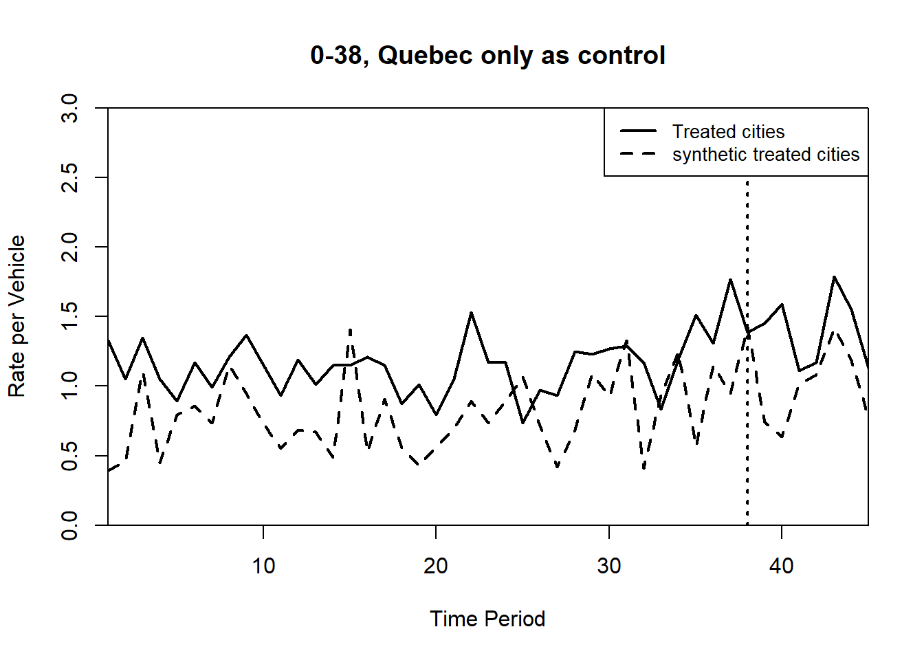
path.plot(synth.res = synth.out_q,dataprep.res = dataprep.out_q,Main="0-38, Quebec only as control",Ylab ="Rate per Vehicle",Xlab ="Time Period",Ylim =c(0,3),Legend =c("Treated cities","synthetic treated cities"),Legend.position ="topright",tr.intake =38)
Code
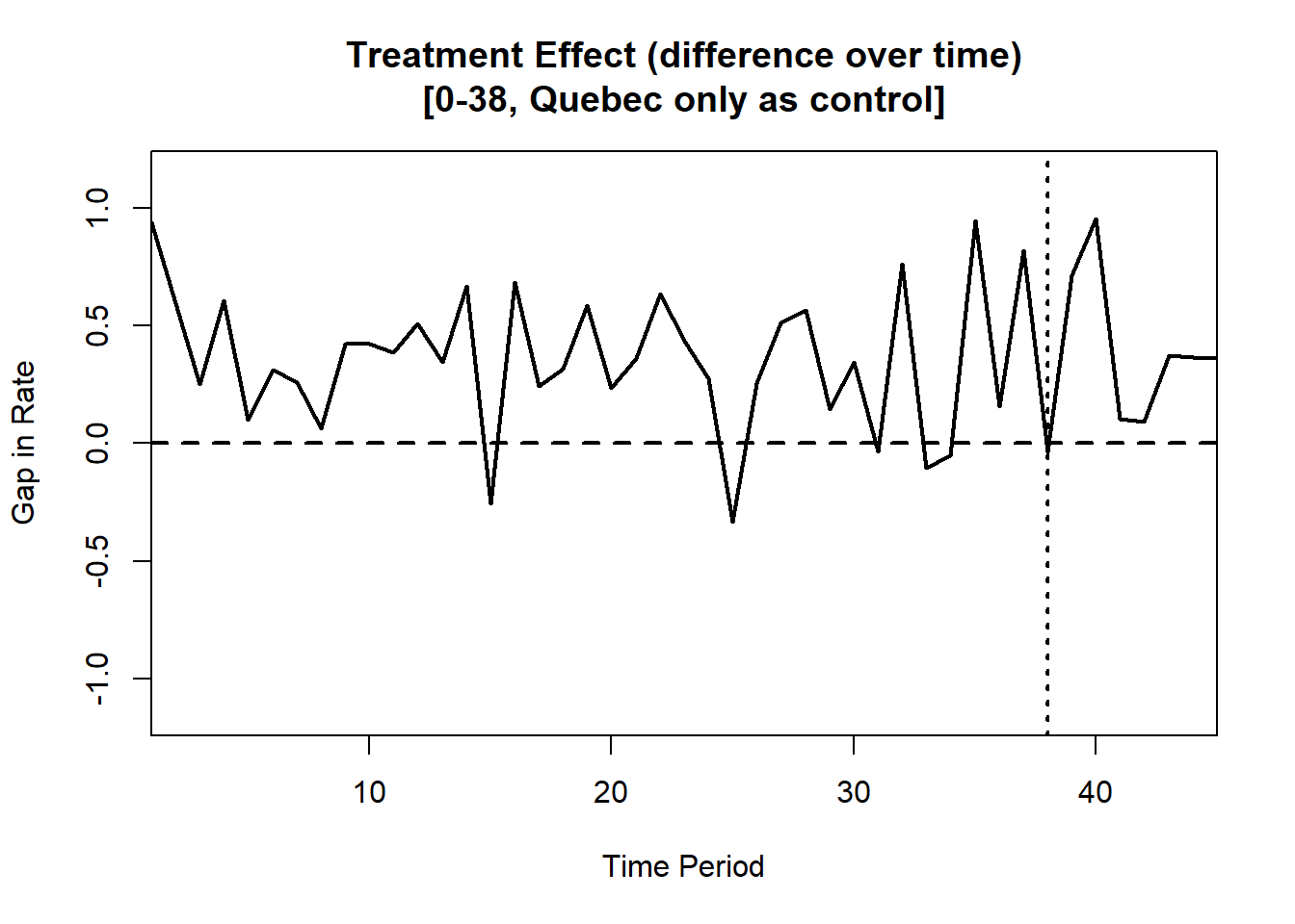
gaps.plot(synth.res = synth.out_q, dataprep.res = dataprep.out_q,Ylab ="Gap in Rate", Xlab ="Time Period",Main ="Treatment Effect (difference over time)\n[0-38, Quebec only as control]",tr.intake =38)
Code
path.plot(synth.res = synth.out,dataprep.res = dataprep.out,Main="0-38, Quebec+Sherbrooke as controls",Ylab ="Rate per Vehicle",Xlab ="Time Period",Ylim =c(0,3),Legend =c("Treated cities","synthetic treated cities"),Legend.position ="topright",tr.intake =38)
Error: objeto 'synth.out' no encontrado
Code
gaps.plot(synth.res = synth.out, dataprep.res = dataprep.out,Ylab ="Gap in Rate", Xlab ="Time Period",Main ="Treatment Effect (difference over time)\n[0-38, Sherbrooke+Quebec as controls]",tr.intake =38)
Error: objeto 'synth.out' no encontrado
Code
cat("**********************************************\n")cat("Placebo tests\n")tdf <- SCtools::generate.placebos(dataprep.out_q,synth.out_q, Sigf.ipop =2) #The Precision setting for the ipop optimization routine. Default of 5.
tdf_sens <- SCtools::generate.placebos(dataprep.out,synth.out, Sigf.ipop =2) #The Precision setting for the ipop optimization routine. Default of 5.
Error: objeto 'synth.out' no encontrado
Code
SCtools::plot_placebos(tdf_sens,title="0-38, Quebec only as control")
Error: objeto 'tdf_sens' no encontrado
Code
SCtools::mspe.test(tdf_sens)$p.val#proportion of ratios of RMSPE, <.05 is significant
Error: objeto 'tdf_sens' no encontrado
Code
SCtools::mspe.plot(tdf = tdf_sens, title="0-38, Quebec only as control\nRatios of RMSPE")
Error: objeto 'tdf_sens' no encontrado
Code
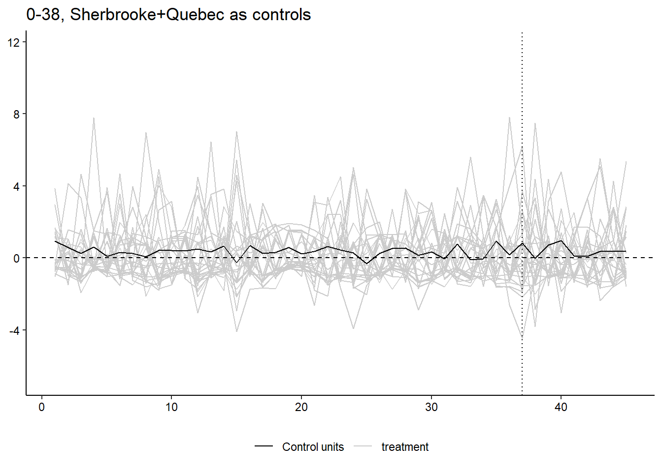
SCtools::plot_placebos(tdf,title="0-38, Sherbrooke+Quebec as controls")
Code
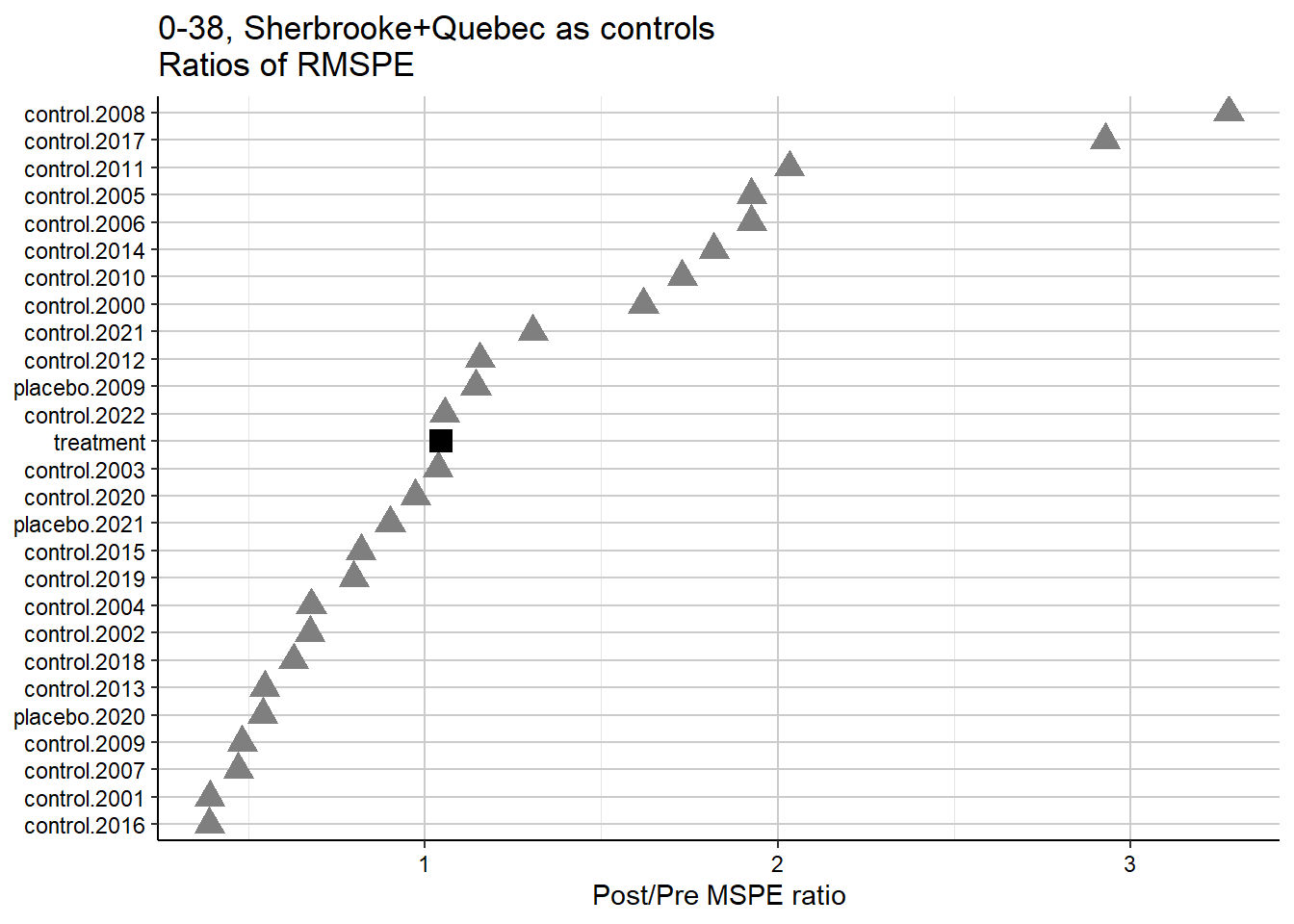
SCtools::mspe.test(tdf)$p.val #proportion of ratios of RMSPE, <.05 is significantSCtools::mspe.plot(tdf = tdf, title="0-38, Sherbrooke+Quebec as controls\nRatios of RMSPE")
Parameters
Print ID labs with treatmentAdded the Lag Y by status and year:
*************************************
0, 38, Quebec+Sherbrooke as controls

X1, X0, Z1, Z0 all come directly from dataprep object.


****************
 searching for synthetic control unit

*************************************
0, 38, Quebec only as controls
For quebec only as a control

X1, X0, Z1, Z0 all come directly from dataprep object.


****************
 searching for synthetic control unit


****************
****************
****************

MSPE (LOSS V): 0.2192477

solution.v:
 0.0002615641 0.3865379 0.2946344 0.3185662

solution.w:
 0.02012723 0.01939688 0.01791392 0.0183393 0.01962153 0.01664269 0.0260252 0.0185402 0.01694998 0.01665177 0.02043387 0.02541825 0.02796451 0.02790998 0.02061454 0.01858557 0.02268817 0.01721553 0.01878756 0.01787663 0.01482893 0.1047135 0.199546 0.02159321 0.01561159 0.2360035

$solution.v
     mean_min_temp_mean_lin mean_max_temp_mean_lin
BFGS           0.0002615641              0.3865379
     mean_median_total_precip_median_lin mean_median_lag_2_prec_median_imp
BFGS                           0.2946344                         0.3185662

$solution.w
     w.weight
1  0.02012723
2  0.01939688
3  0.01791392
4  0.01833930
5  0.01962153
6  0.01664269
7  0.02602520
8  0.01854020
9  0.01694998
10 0.01665177
11 0.02043387
12 0.02541825
13 0.02796451
14 0.02790998
15 0.02061454
16 0.01858557
17 0.02268817
18 0.01721553
19 0.01878756
20 0.01787663
21 0.01482893
22 0.10471349
23 0.19954601
24 0.02159321
25 0.01561159
26 0.23600346

$loss.v
          46
46 0.2192477

$loss.w
            w.weight
w.weight 0.000107966

$custom.v
NULL

$rgV.optim
$rgV.optim$out.list
                      p1         p2       p3         p4     value fevals gevals
BFGS        0.0004034702 -0.5962458 0.454482 0.49139749 0.2192477    201     18
Nelder-Mead 0.0764864017  0.1408110 1.126535 0.07522402 0.5254337    439     NA
            niter convcode kkt1 kkt2 xtime
BFGS           NA        0   NA   NA  0.36
Nelder-Mead    NA        0   NA   NA  0.47

$rgV.optim$par
               p1         p2       p3        p4
BFGS 0.0004034702 -0.5962458 0.454482 0.4913975

$rgV.optim$value
[1] 0.2192477


**********************************************
Placebo tests

X1, X0, Z1, Z0 all come directly from dataprep object.


****************
 searching for synthetic control unit


****************
****************
****************

MSPE (LOSS V): 2.362667

solution.v:
 2.44e-08 0.0000120052 0.466436 0.5335519

solution.w:
 0.02610002 0.03786027 0.02347817 0.02820972 0.01660514 0.02165607 0.02490107 0.0230292 0.0230945 0.02673908 0.10015 0.02855692 0.02476013 0.03271842 0.0237351 0.0262851 0.02301282 0.03004343 0.029588 0.01027368 0.3529467 0.02337534 0.0320491 0.01081606 0.0000160716


X1, X0, Z1, Z0 all come directly from dataprep object.


****************
 searching for synthetic control unit


****************
****************
****************

MSPE (LOSS V): 4.650771

solution.v:
 2.8e-08 0.1372447 0.8627547 6.055e-07

solution.w:
 0.0383725 0.03991688 0.03820043 0.03806895 0.03771285 0.04103626 0.0382547 0.03867514 0.03848169 0.03881355 0.03837142 0.03656983 0.0337973 0.03810089 0.03824008 0.03740278 0.03825246 0.03835981 0.03929635 0.03783707 0.04144968 0.03442201 0.03818963 0.03949361 0.08268551


X1, X0, Z1, Z0 all come directly from dataprep object.


****************
 searching for synthetic control unit


****************
****************
****************

MSPE (LOSS V): 5.919042

solution.v:
 5e-09 0.0002108255 0.4877529 0.5120362

solution.w:
 0.0333778 0.02343195 0.02173179 0.0248291 0.02257851 0.02259581 0.02298457 0.02319133 0.02218131 0.02453149 0.3781012 0.02601698 0.04365524 0.03088031 0.02154274 0.02278146 0.02347481 0.02652422 0.02728331 0.02245965 0.04205549 0.02193005 0.02842275 0.02194683 0.02149132


X1, X0, Z1, Z0 all come directly from dataprep object.


****************
 searching for synthetic control unit


****************
****************
****************

MSPE (LOSS V): 4.927495

solution.v:
 3e-10 1 0 0

solution.w:
 0.04587076 0.03161901 0.1956664 0.04282516 0.04251878 0.01628168 0.03166438 0.05345027 0.04685743 0.02449315 0.04560612 0.03148304 0.03816531 0.03440298 0.02703455 0.03024543 0.04563255 0.02922233 0.06326866 0.02671056 0.01556565 0.02461973 0.03576921 0.01960071 0.001425787


X1, X0, Z1, Z0 all come directly from dataprep object.


****************
 searching for synthetic control unit


****************
****************
****************

MSPE (LOSS V): 2.585146

solution.v:
 1.6e-09 0.5602369 3.25e-08 0.439763

solution.w:
 0.04255902 0.02788961 0.08695119 0.04292756 0.03388969 0.0134891 0.02742241 0.04815552 0.04246243 0.02097712 0.04443389 0.03301185 0.2006433 0.02981539 0.0243421 0.02979844 0.03944401 0.02580755 0.07916953 0.01994622 0.01285458 0.02563449 0.03290261 0.01448177 0.0009748869


X1, X0, Z1, Z0 all come directly from dataprep object.


****************
 searching for synthetic control unit


****************
****************
****************

MSPE (LOSS V): 4.487183

solution.v:
 0.2024038 0.704045 2.5e-09 0.09355117

solution.w:
 0.04234068 0.01909945 0.03611808 0.02356999 0.01528563 0.103269 0.01958211 0.2439891 0.02819108 0.01369887 0.2124013 0.008280413 0.004731603 0.02465725 0.01059163 0.01101023 0.05587113 0.006300628 0.02165539 0.01749989 0.00543159 0.006183711 0.02160002 0.0348654 0.01376928


X1, X0, Z1, Z0 all come directly from dataprep object.


****************
 searching for synthetic control unit


****************
****************
****************

MSPE (LOSS V): 5.268936

solution.v:
 0.001434662 4.98e-08 0.470981 0.5275843

solution.w:
 0.02597885 0.02592471 0.02319121 0.02379551 0.0214001 0.02666481 0.02632666 0.02670973 0.02544762 0.02668663 0.02535671 0.01849385 0.0125674 0.02647004 0.02468303 0.02140143 0.02687757 0.02434914 0.02095293 0.01832076 0.02514607 0.01652828 0.02508251 0.02095524 0.4406893


X1, X0, Z1, Z0 all come directly from dataprep object.


****************
 searching for synthetic control unit


****************
****************
****************

MSPE (LOSS V): 4.231985

solution.v:
 0.1024347 0.02722927 0.8703358 1.79e-07

solution.w:
 0.04089896 0.03890509 0.04513533 0.0336339 0.03573922 0.04607023 0.03587961 0.04374974 0.0427716 0.04141597 0.03871521 0.02882638 0.02305805 0.04291571 0.03702117 0.0315364 0.04433664 0.0447376 0.03986249 0.05648059 0.05228785 0.02311006 0.03766141 0.04799044 0.04726213


X1, X0, Z1, Z0 all come directly from dataprep object.


****************
 searching for synthetic control unit


****************
****************
****************

MSPE (LOSS V): 2.407

solution.v:
 0.07901008 0.0139081 0.5325692 0.3745126

solution.w:
 0.02805138 0.02252407 0.1237155 0.02247622 0.02104275 0.1539677 0.01595562 0.02462436 0.04988874 0.021222 0.02077843 0.01368858 0.01000343 0.02472665 0.0205673 0.01607445 0.05912815 0.02376243 0.03356237 0.1891534 0.02128401 0.01029167 0.02078275 0.03758727 0.01514107


X1, X0, Z1, Z0 all come directly from dataprep object.


****************
 searching for synthetic control unit


****************
****************
****************

MSPE (LOSS V): 3.147491

solution.v:
 0.009263263 0.009711711 0.7781159 0.2029091

solution.w:
 0.02043191 0.02697304 0.1352807 0.03713078 0.03361861 0.0297932 0.01842804 0.02925483 0.1052986 0.02200648 0.01480252 0.02217827 0.02009186 0.0186525 0.03364594 0.02559236 0.04734124 0.02878289 0.08433248 0.1540339 0.01244773 0.02013912 0.02201726 0.01987046 0.01785552


X1, X0, Z1, Z0 all come directly from dataprep object.


****************
 searching for synthetic control unit


****************
****************
****************

MSPE (LOSS V): 2.013816

solution.v:
 0.9471962 4.55e-08 0.05280033 0.0000034351

solution.w:
 0.0393264 0.03860363 0.04073954 0.03604726 0.03749065 0.04176211 0.05419832 0.03913182 0.04015905 0.03994095 0.03891602 0.03373993 0.03049256 0.04006617 0.03793038 0.03521746 0.04037772 0.04064201 0.03934566 0.0430041 0.04249067 0.02913003 0.03808784 0.04349016 0.05967075


X1, X0, Z1, Z0 all come directly from dataprep object.


****************
 searching for synthetic control unit


****************
****************
****************

MSPE (LOSS V): 2.173148

solution.v:
 0.02593841 0.08459036 0.6433283 0.2461429

solution.w:
 0.09494028 0.03065182 0.1189216 0.03427309 0.03084698 0.09125986 0.03671708 0.02949425 0.05978163 0.03075634 0.02779792 0.02546431 0.02183486 0.04825039 0.02280236 0.02552512 0.04767017 0.0242323 0.03811706 0.02125396 0.02915513 0.01953511 0.04192641 0.02822888 0.02056632


X1, X0, Z1, Z0 all come directly from dataprep object.


****************
 searching for synthetic control unit


****************
****************
****************

MSPE (LOSS V): 1.793304

solution.v:
 0.3233482 0.5578955 0.1124072 0.006349065

solution.w:
 0.02960555 0.02760306 0.03653661 0.03154717 0.0358836 0.02617807 0.007321828 0.02762839 0.03144258 0.03273988 0.02469504 0.02816388 0.05968285 0.0268853 0.02924407 0.03046909 0.02972756 0.03031499 0.03936313 0.02393107 0.0197512 0.3249028 0.0282354 0.01814933 -0.0000193706


X1, X0, Z1, Z0 all come directly from dataprep object.


****************
 searching for synthetic control unit


****************
****************
****************

MSPE (LOSS V): 1.447422

solution.v:
 0.5449023 0.4270488 0.0228453 0.005203676

solution.w:
 0.02542083 0.01898451 0.07875129 0.0255609 0.05211937 0.01970534 0.003636155 0.01992187 0.03458103 0.04002946 0.01494921 0.0193806 0.0352086 0.01991919 0.02009461 0.01944919 0.02849029 0.02923249 0.113906 0.01907247 0.01119471 0.3186891 0.01958357 0.009613728 0.002503711


X1, X0, Z1, Z0 all come directly from dataprep object.


****************
 searching for synthetic control unit


****************
****************
****************

MSPE (LOSS V): 1.032805

solution.v:
 0.5161918 0 0.4838082 0

solution.w:
 0.03103054 0.02870619 0.03597049 0.0221264 0.0256797 0.04241195 0.01751479 0.03072191 0.03536468 0.03378832 0.03233972 0.02710506 0.01838356 0.01379155 0.02698256 0.02075487 0.03651665 0.03629074 0.0301654 0.1719755 0.05775756 0.01271351 0.02679527 0.05284151 0.1322716


X1, X0, Z1, Z0 all come directly from dataprep object.


****************
 searching for synthetic control unit


****************
****************
****************

MSPE (LOSS V): 1.105641

solution.v:
 0.003870062 0.02811751 0.6557904 0.312222

solution.w:
 0.02050621 0.02872594 0.02396753 0.03798631 0.03000329 0.02874093 0.01253822 0.03136052 0.03040579 0.03895509 0.02479317 0.01501946 0.02266849 0.05388658 0.02032724 0.0322666 0.02945465 0.02927848 0.02945757 0.03873454 0.01396273 0.182649 0.02114795 0.03143203 0.1717318


X1, X0, Z1, Z0 all come directly from dataprep object.


****************
 searching for synthetic control unit


****************
****************
****************

MSPE (LOSS V): 1.554308

solution.v:
 0.6605057 0.00829095 0.000021836 0.3311815

solution.w:
 0.02658709 0.027252 0.02474225 0.02790006 0.0267382 0.02489566 0.0422964 0.02677158 0.02512797 0.02531664 0.02724012 0.02819688 0.03125796 0.2344396 0.02669795 0.02743914 0.02536595 0.02589762 0.02510602 0.02449656 0.02658123 0.1363043 0.02787613 0.02586965 0.0296031


X1, X0, Z1, Z0 all come directly from dataprep object.


****************
 searching for synthetic control unit


****************
****************
****************

MSPE (LOSS V): 0.8981232

solution.v:
 0.5345049 1.5e-09 3.55e-08 0.465495

solution.w:
 0.02552694 0.02556272 0.02057838 0.02408872 0.02437274 0.02790759 0.02541059 0.02563492 0.02430484 0.0217773 0.02587332 0.02369909 0.02031106 0.01533852 0.02582109 0.02519089 0.02263616 0.02056639 0.0231166 0.4240628 0.02471809 0.0151167 0.02482896 0.03015918 0.03339644


X1, X0, Z1, Z0 all come directly from dataprep object.


****************
 searching for synthetic control unit


****************
****************
****************

MSPE (LOSS V): 0.8533204

solution.v:
 0.1542203 0.05150248 0.3023669 0.4919103

solution.w:
 0.01325394 0.01682898 -0.0000027626 0.01271502 0.02177555 0.01132166 0.007771834 0.01788792 0.01201838 0.01743443 0.0200416 0.01159097 0.01563805 0.01440415 0.01637431 0.02266615 0.01600169 0.01360041 0.3623555 0.2832141 0.04451018 0.009348225 0.01472632 0.01382535 0.01069928


X1, X0, Z1, Z0 all come directly from dataprep object.


****************
 searching for synthetic control unit


****************
****************
****************

MSPE (LOSS V): 3.451762

solution.v:
 6.7e-09 0.114019 0.7904737 0.0955073

solution.w:
 0.01816032 0.01164339 0.5061552 0.02126276 0.02075419 0.0147375 0.005126241 0.01146825 0.0230167 0.02016538 0.008234151 0.01771211 0.01425117 0.2022179 0.0119647 0.01022716 0.01278527 0.01762982 0.01034836 0.007937283 0.004415225 0.01010924 0.01371846 0.005614843 0.0003432345


X1, X0, Z1, Z0 all come directly from dataprep object.


****************
 searching for synthetic control unit


****************
****************
****************

MSPE (LOSS V): 0.439976

solution.v:
 0.01439672 0.01659347 0.1309774 0.8380324

solution.w:
 0.006315433 0.005798133 0.01040409 0.004102556 0.003939236 0.0000940843 0.004086438 0.006826619 0.0135721 0.01145107 0.006646598 0.004444653 0.002057792 0.0008037353 0.007202124 0.005133568 0.002934014 0.01323293 0.008940676 0.005596583 0.01282482 0.001325226 0.004765199 0.7143724 0.1431299


X1, X0, Z1, Z0 all come directly from dataprep object.


****************
 searching for synthetic control unit


****************
****************
****************

MSPE (LOSS V): 0.8465404

solution.v:
 0.3105285 0.5380839 0.004586739 0.1468009

solution.w:
 0.02173792 0.02940965 0.02270297 0.02059237 0.02736386 0.02238186 0.01368448 0.03133883 0.02322982 0.02950166 0.0367941 0.01780915 0.0234833 0.01825865 0.0282247 0.03679333 0.02599037 0.0257923 0.05140511 0.02561732 0.05495722 0.01715595 0.02443543 0.03304987 0.3382658


X1, X0, Z1, Z0 all come directly from dataprep object.


****************
 searching for synthetic control unit


****************
****************
****************

MSPE (LOSS V): 1.005965

solution.v:
 1e-10 1 1e-10 1e-10

solution.w:
 0.02960233 0.03082939 0.02658361 0.0298276 0.02991553 0.02994594 0.03059864 0.03082678 0.02876582 0.02949719 0.03106181 0.02963026 0.03083714 0.03035089 0.03064929 0.03102482 0.03090264 0.02962747 0.03094953 0.02770606 0.03103278 0.03049254 0.03054747 0.03092461 0.2778672


X1, X0, Z1, Z0 all come directly from dataprep object.


****************
 searching for synthetic control unit


****************
****************
****************

MSPE (LOSS V): 0.5678277

solution.v:
 0.3972689 0.5773889 0.02531761 0.0000245207

solution.w:
 0.04893186 0.03369509 0.0481924 0.04815142 0.03629803 0.05167266 0.148415 0.03265335 0.0491855 0.0383633 0.02680714 0.05836209 0.03361832 0.0372436 0.03656618 0.02672861 0.03282717 0.04377628 0.02256334 0.04126178 0.02373792 0.01728152 0.03556991 0.0280994 -0.0000064714


X1, X0, Z1, Z0 all come directly from dataprep object.


****************
 searching for synthetic control unit


****************
****************
****************

MSPE (LOSS V): 0.2727189

solution.v:
 0.002636212 0.01237997 0.0002803692 0.9847034

solution.w:
 0.006726814 0.0066493 0.005740253 0.005458335 0.004506097 0.0000109181 0.00890502 0.007045174 0.007311515 0.006897839 0.007207516 0.005870622 0.003100356 0.001420714 0.007196162 0.006008251 0.004218158 0.007547347 0.006301385 0.004633662 0.4161386 0.0081095 0.002412846 0.005977656 0.454606


X1, X0, Z1, Z0 all come directly from dataprep object.


****************
 searching for synthetic control unit


****************
****************
****************

MSPE (LOSS V): 0.248964

solution.v:
 4.1e-09 0.09172457 0.452561 0.4557145

solution.w:
 0.005650323 0.006684122 0.004143104 0.004545757 0.004136676 0.005904232 0.01401961 0.007023068 0.00543199 0.005547505 0.008603769 0.00537549 0.003270773 0.001321492 0.007105716 0.00640486 0.004380614 0.00606954 0.007089397 0.00364449 0.0000167814 0.01982559 0.002544936 0.005860097 0.8554

[1] 0.4814815
The pre-treatment balance diagnostics show an excellent fit between treated and its synthetic control. The absolute gaps in the main predictors translate into relative differences of ≤ 10 %. Crucially, the two variables that receive virtually all the weight in the V-matrix—current precipitation and precipitation lagged two days—match almost perfectly (≤ 0.3 % gap), as does the 10-day lag of the outcome. Overall, the synthetic control replicates the treated unit’s pre-grand prix trajectory very closely, so the absence of a post-event divergence cannot be attributed to poor pre-treatment balance.*
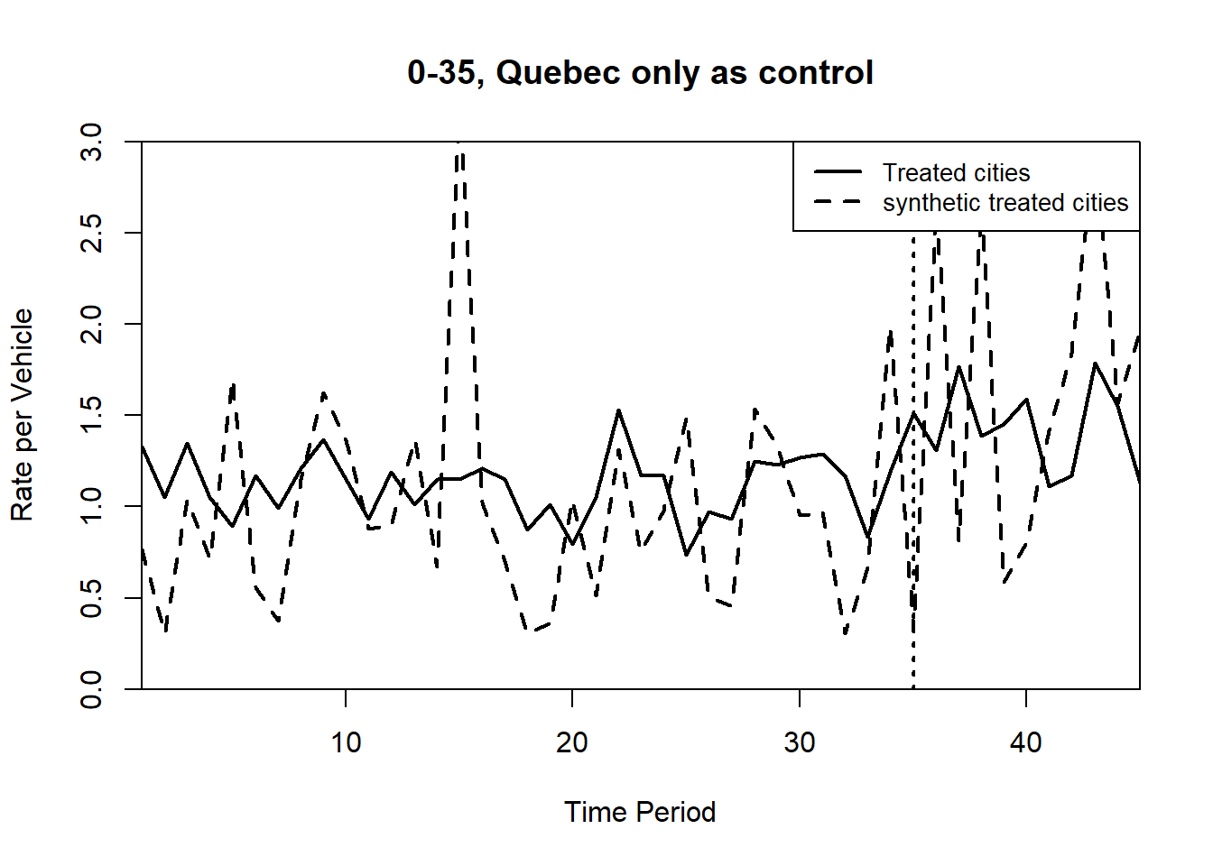
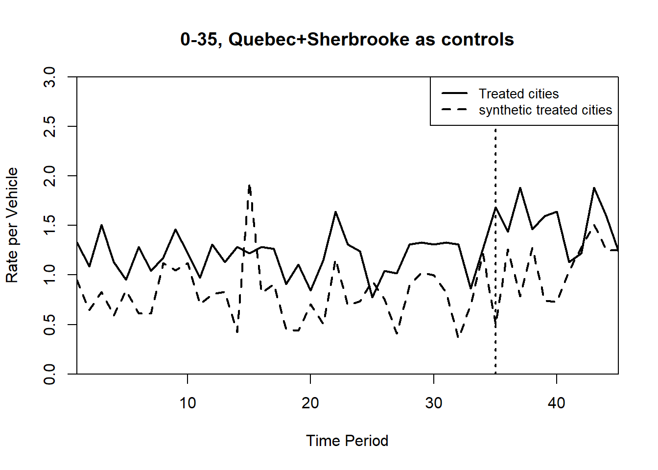
Units 6, 7, 14, 20 explain more than 97% of the synthetic control (w.weights). For Quebec only as controls, donor units 7, 15, 6, 20, 2 explain 79% of the synthetic control.
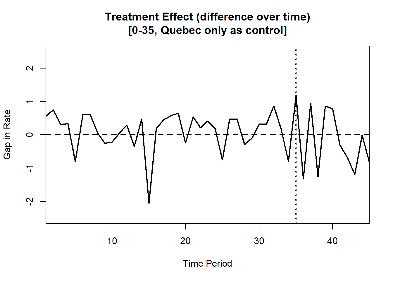
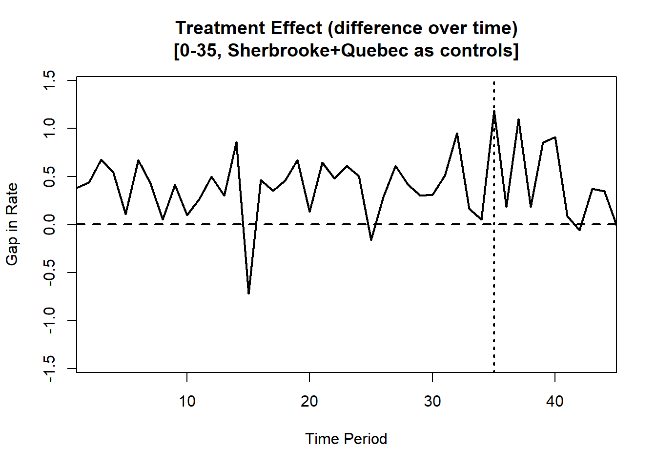
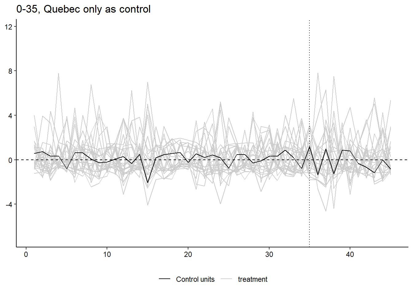
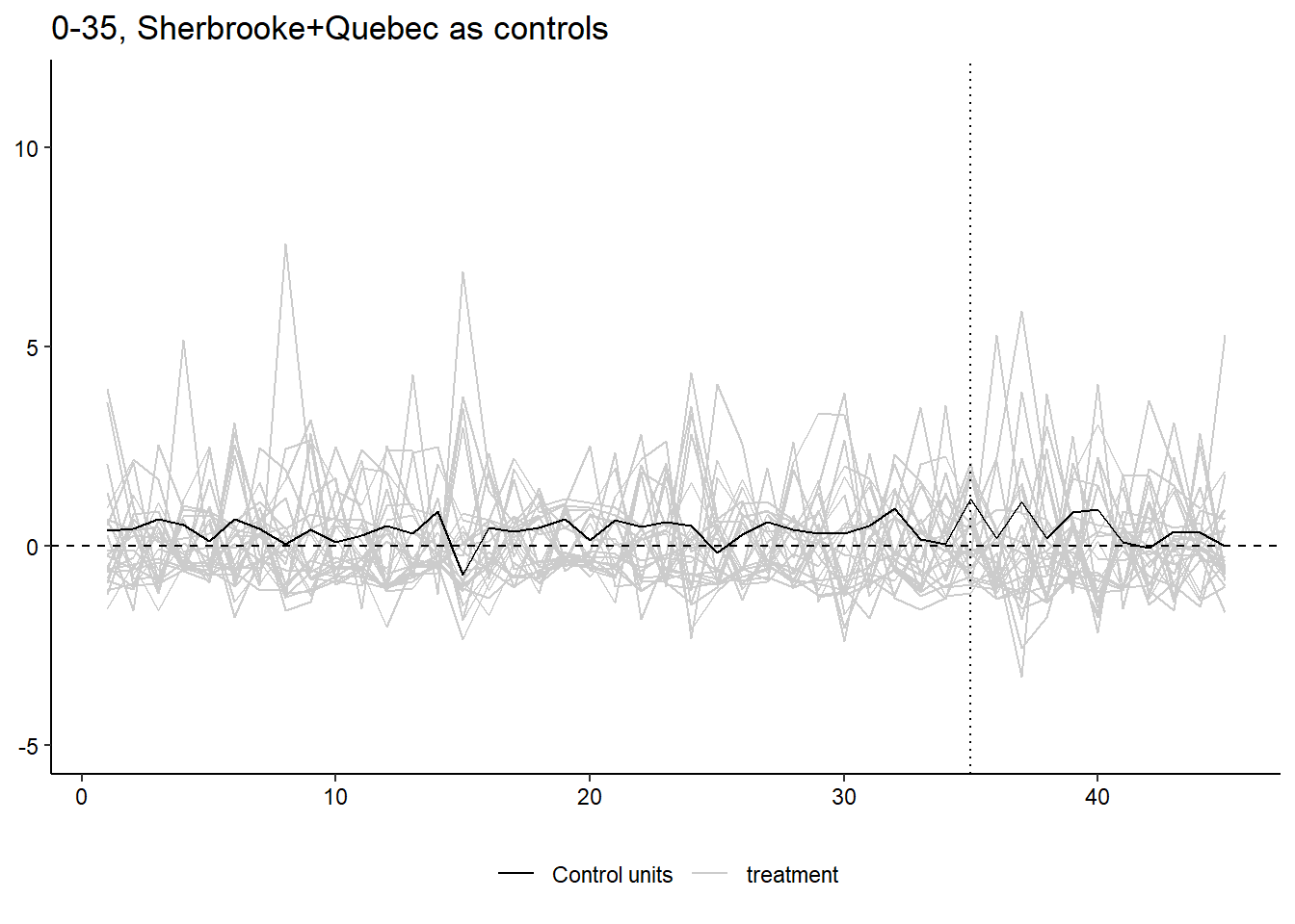
The effect post Grand Prix does not differentiate compared to the pseudo-treated units. There is no evidence of an unusual causal effect.
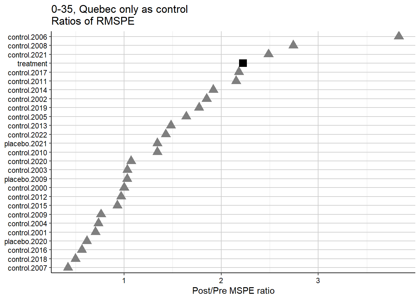
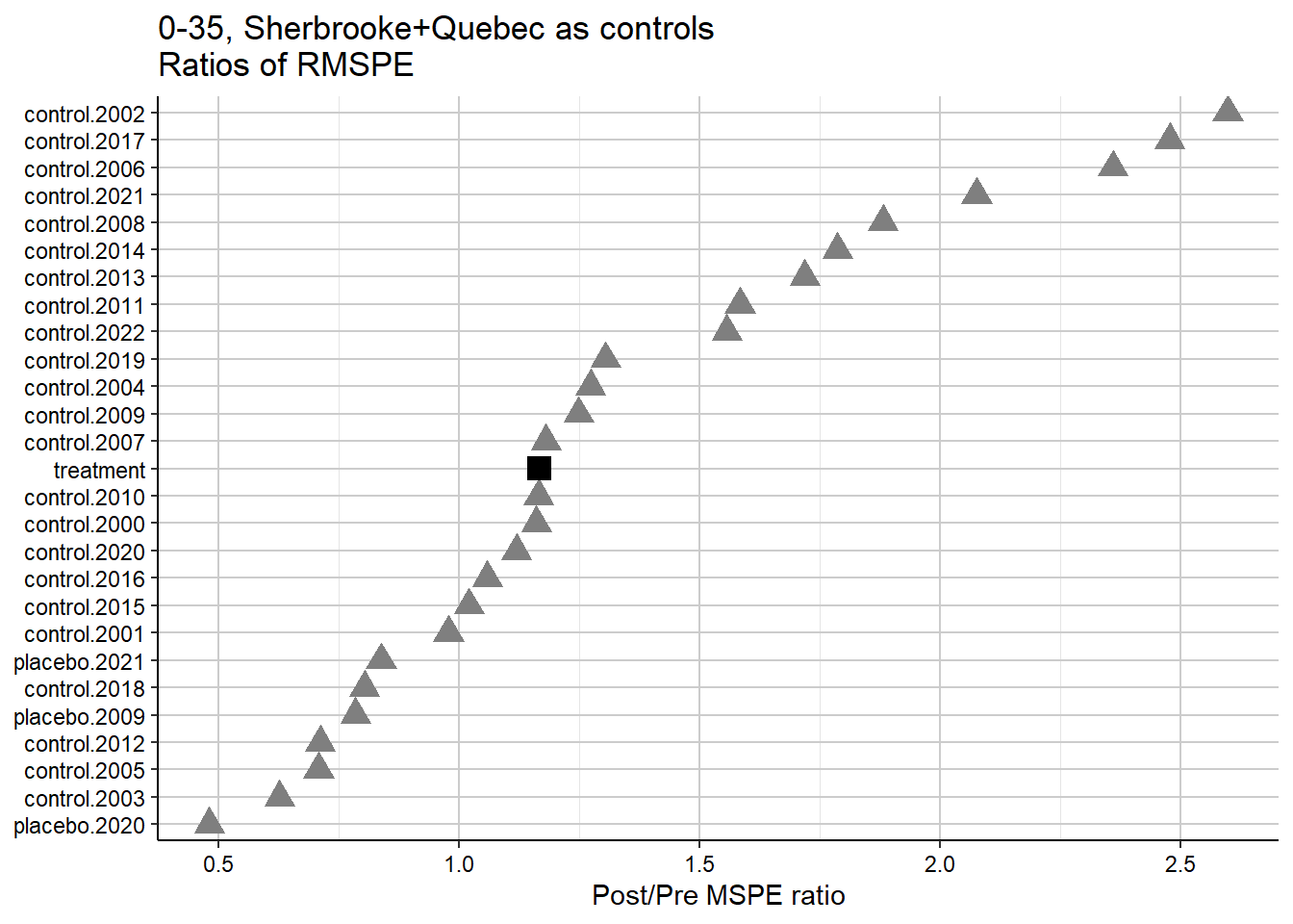
Ratios of RMSPE (root mean squared prediction errors) post/pre-intervention and the proportion of control units with ratios greater or equal to treated does not detect a causal effect.
We replicated the analysis with the intervention period 2 days before the race.
Code
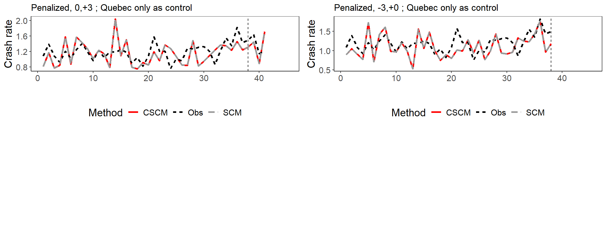
if(identical(collisions_weather_corr$total_precip_median_lin, collisions_weather_corr$lag_2_prec_median_lin)){stop("The variable was not lagged")}collisions_weather_corr_rect_synth_one_tr_many_cntrls |>filter(is.na(Y_lag10)) |>nrow()collisions_weather_corr_rect_quebec_synth_one_tr_many_cntrls |>filter(is.na(Y_lag10)) |>nrow()collisions_weather_corr_rect_synth_one_tr_many_cntrls$id <-as.numeric(collisions_weather_corr_rect_synth_one_tr_many_cntrls$id)collisions_weather_corr_rect_quebec_synth_one_tr_many_cntrls$id <-as.numeric(collisions_weather_corr_rect_quebec_synth_one_tr_many_cntrls$id)if(max(collisions_weather_corr_rect_synth_one_tr_many_cntrls$rate_veh)<1){collisions_weather_corr_rect_synth_one_tr_many_cntrls$rate_veh <- collisions_weather_corr_rect_synth_one_tr_many_cntrls$rate_veh*10}if(max(collisions_weather_corr_rect_quebec_synth_one_tr_many_cntrls$rate_veh)<1){collisions_weather_corr_rect_quebec_synth_one_tr_many_cntrls$rate_veh <- collisions_weather_corr_rect_quebec_synth_one_tr_many_cntrls$rate_veh*10}collisions_weather_corr_rect_synth_one_tr_many_cntrls<-data.frame(collisions_weather_corr_rect_synth_one_tr_many_cntrls)collisions_weather_corr_rect_quebec_synth_one_tr_many_cntrls<-data.frame(collisions_weather_corr_rect_quebec_synth_one_tr_many_cntrls)##:#:#:#::#:#:#:#:##:#:#:#::#:#:#:#:##:#:#:#::#:#:#:#:##:#:#:#::#:#:#:#:##:#:#:#::#:#:#:#:##:#:#:#::#:#:#:#:##:#:#:#::#:#:#:#:##:#:#:#::#:#:#:#:##:#:#:#::#:#:#:#:##:#:#:#::#:#:#:#:##:#:#:#::#:#:#:#:##:#:#:#::#:#:#:#:cat("*************************************\n")cat("0, 35, Quebec+Sherbrooke as controls\n")dataprep.out2 <- Synth::dataprep(foo = collisions_weather_corr_rect_synth_one_tr_many_cntrls,predictors =c("mean_min_temp_mean_lin", "mean_max_temp_mean_lin", "mean_median_total_precip_median_lin", "mean_median_lag_2_prec_median_imp"),dependent ="rate_veh",unit.variable ="id",time.variable ="yday_corr",treatment.identifier =46, # Laval, Montreal, Longueuilcontrols.identifier =1:26,time.predictors.prior =1:(t_int_man-3), #nates tenía menos 1time.optimize.ssr =1:(t_int_man-3),time.plot=1:max_time,unit.names.variable ="id_lab")synth.out2 <-synth(dataprep.out2, method ="BFGS")print(synth.out2)gaps2 <- dataprep.out2$Y1plot - (dataprep.out2$Y0plot %*% synth.out2$solution.w)synth.tables2 <-synth.tab(dataprep.res = dataprep.out2,synth.res = synth.out2 )cat("*************************************\n")cat("0, 35, Quebec only as control\n")dataprep.out2_q <- Synth::dataprep(foo = collisions_weather_corr_rect_quebec_synth_one_tr_many_cntrls,predictors =c("mean_min_temp_mean_lin", "mean_max_temp_mean_lin", "mean_median_total_precip_median_lin", "mean_median_lag_2_prec_median_imp"),dependent ="rate_veh",unit.variable ="id",time.variable ="yday_corr",treatment.identifier =46, # Laval, Montreal, Longueuilcontrols.identifier =1:26,time.predictors.prior =1:(t_int_man-3),time.optimize.ssr =1:(t_int_man-3),time.plot=1:max_time,unit.names.variable ="id_lab")synth.out2_q <-synth(dataprep.out2_q, method ="BFGS")print(synth.out2_q)gaps2_q <- dataprep.out2_q$Y1plot - (dataprep.out2_q$Y0plot %*% synth.out2_q$solution.w)synth.tables2_q <-synth.tab(dataprep.res = dataprep.out2_q,synth.res = synth.out2_q )rbind.data.frame(cbind.data.frame(type="0-35, Quebec+Sherbrooke as controls",synth.tables2$tab.pred, predictor_weight=synth.tables2$tab.v), cbind.data.frame(type="0-35, Quebec only as control",synth.tables2_q$tab.pred, predictor_weight=synth.tables2_q$tab.v))|>mutate(`Sample Mean`=sprintf("%1.2f",`Sample Mean`), v.weights=sprintf("%1.2f",v.weights), abs_diff=sprintf("%1.2f",abs(Treated-Synthetic)), ratio=sprintf("%1.2f",Treated/Synthetic), gap_pct_ctrl=sprintf("%1.2f", abs(100*(Treated-Synthetic)/Synthetic)))|> knitr::kable("markdown", caption="Comparison of pre-treatment predictor values for treated unit, synthetic control and all units in the sample")rbind.data.frame(cbind.data.frame(type="0-35, Quebec+Sherbrooke as controls", synth.tables2$tab.w), cbind.data.frame(type="0-35, Quebec only as control", synth.tables2_q$tab.w))|>arrange(type, desc(w.weights))|> knitr::kable("markdown", caption="Weight for each potential control unit")path.plot(synth.res = synth.out2_q,dataprep.res = dataprep.out2_q,Main="0-35, Quebec only as control",Ylab ="Rate per Vehicle",Xlab ="Time Period",Ylim =c(0,3),Legend =c("Treated cities","synthetic treated cities"),Legend.position ="topright",tr.intake =38-3)
Code
gaps.plot(synth.res = synth.out2_q, dataprep.res = dataprep.out2_q,Ylab ="Gap in Rate", Xlab ="Time Period",Main ="Treatment Effect (difference over time)\n[0-35, Quebec only as control]",tr.intake =38-3)
Code
path.plot(synth.res = synth.out2,dataprep.res = dataprep.out2,Main="0-35, Quebec+Sherbrooke as controls",Ylab ="Rate per Vehicle",Xlab ="Time Period",Ylim =c(0,3),Legend =c("Treated cities","synthetic treated cities"),Legend.position ="topright",tr.intake =38-3)
Code
gaps.plot(synth.res = synth.out2, dataprep.res = dataprep.out2,Ylab ="Gap in Rate", Xlab ="Time Period",Main ="Treatment Effect (difference over time)\n[0-35, Sherbrooke+Quebec as controls]",tr.intake =38-3)
Code
cat("**********************************************\n")cat("Placebo tests\n")tdf2_q <- SCtools::generate.placebos(dataprep.out2_q,synth.out2_q, Sigf.ipop =2) #The Precision setting for the ipop optimization routine. Default of 5.
Comparison of pre-treatment predictor values for treated unit, synthetic control and all units in the sample
type
Treated
Synthetic
Sample Mean
v.weights
abs_diff
ratio
gap_pct_ctrl
mean_min_temp_mean_lin
0-35, Quebec+Sherbrooke as controls
9.584
8.491
7.11
0.00
1.09
1.13
12.87
mean_max_temp_mean_lin
0-35, Quebec+Sherbrooke as controls
20.437
20.437
19.17
0.11
0.00
1.00
0.00
mean_median_total_precip_median_lin
0-35, Quebec+Sherbrooke as controls
2.895
2.895
3.00
0.34
0.00
1.00
0.00
mean_median_lag_2_prec_median_imp
0-35, Quebec+Sherbrooke as controls
2.950
2.950
3.09
0.55
0.00
1.00
0.00
mean_min_temp_mean_lin1
0-35, Quebec only as control
8.942
8.942
6.91
0.28
0.00
1.00
0.00
mean_max_temp_mean_lin1
0-35, Quebec only as control
20.152
20.153
18.72
0.09
0.00
1.00
0.00
mean_median_total_precip_median_lin1
0-35, Quebec only as control
2.887
2.886
2.89
0.31
0.00
1.00
0.03
mean_median_lag_2_prec_median_imp1
0-35, Quebec only as control
2.952
2.953
2.97
0.32
0.00
1.00
0.03
Weight for each potential control unit
type
w.weights
unit.names
unit.numbers
71
0-35, Quebec only as control
0.239
control.2006
7
231
0-35, Quebec only as control
0.208
control.2022
23
261
0-35, Quebec only as control
0.198
placebo.2021
26
121
0-35, Quebec only as control
0.114
control.2011
12
41
0-35, Quebec only as control
0.037
control.2003
4
61
0-35, Quebec only as control
0.017
control.2005
6
110
0-35, Quebec only as control
0.015
control.2000
1
91
0-35, Quebec only as control
0.014
control.2008
9
131
0-35, Quebec only as control
0.014
control.2012
13
181
0-35, Quebec only as control
0.013
control.2017
18
241
0-35, Quebec only as control
0.013
placebo.2009
24
141
0-35, Quebec only as control
0.012
control.2013
14
31
0-35, Quebec only as control
0.011
control.2002
3
51
0-35, Quebec only as control
0.011
control.2004
5
171
0-35, Quebec only as control
0.011
control.2016
17
201
0-35, Quebec only as control
0.011
control.2019
20
27
0-35, Quebec only as control
0.010
control.2001
2
101
0-35, Quebec only as control
0.010
control.2009
10
151
0-35, Quebec only as control
0.010
control.2014
15
81
0-35, Quebec only as control
0.009
control.2007
8
111
0-35, Quebec only as control
0.006
control.2010
11
161
0-35, Quebec only as control
0.005
control.2015
16
191
0-35, Quebec only as control
0.004
control.2018
19
211
0-35, Quebec only as control
0.004
control.2020
21
251
0-35, Quebec only as control
0.003
placebo.2020
25
221
0-35, Quebec only as control
0.000
control.2021
22
26
0-35, Quebec+Sherbrooke as controls
0.218
placebo.2021
26
23
0-35, Quebec+Sherbrooke as controls
0.133
control.2022
23
7
0-35, Quebec+Sherbrooke as controls
0.112
control.2006
7
12
0-35, Quebec+Sherbrooke as controls
0.028
control.2011
12
13
0-35, Quebec+Sherbrooke as controls
0.028
control.2012
13
17
0-35, Quebec+Sherbrooke as controls
0.028
control.2016
17
16
0-35, Quebec+Sherbrooke as controls
0.026
control.2015
16
24
0-35, Quebec+Sherbrooke as controls
0.026
placebo.2009
24
4
0-35, Quebec+Sherbrooke as controls
0.025
control.2003
4
5
0-35, Quebec+Sherbrooke as controls
0.025
control.2004
5
8
0-35, Quebec+Sherbrooke as controls
0.025
control.2007
8
1
0-35, Quebec+Sherbrooke as controls
0.024
control.2000
1
2
0-35, Quebec+Sherbrooke as controls
0.024
control.2001
2
11
0-35, Quebec+Sherbrooke as controls
0.024
control.2010
11
15
0-35, Quebec+Sherbrooke as controls
0.024
control.2014
15
20
0-35, Quebec+Sherbrooke as controls
0.024
control.2019
20
3
0-35, Quebec+Sherbrooke as controls
0.023
control.2002
3
9
0-35, Quebec+Sherbrooke as controls
0.023
control.2008
9
10
0-35, Quebec+Sherbrooke as controls
0.023
control.2009
10
18
0-35, Quebec+Sherbrooke as controls
0.023
control.2017
18
6
0-35, Quebec+Sherbrooke as controls
0.022
control.2005
6
14
0-35, Quebec+Sherbrooke as controls
0.022
control.2013
14
19
0-35, Quebec+Sherbrooke as controls
0.021
control.2018
19
21
0-35, Quebec+Sherbrooke as controls
0.020
control.2020
21
25
0-35, Quebec+Sherbrooke as controls
0.019
placebo.2020
25
22
0-35, Quebec+Sherbrooke as controls
0.012
control.2021
22
**********************************************
Placebo tests

X1, X0, Z1, Z0 all come directly from dataprep object.


****************
 searching for synthetic control unit


****************
****************
****************

MSPE (LOSS V): 2.929933

solution.v:
 0.02701167 0.06371052 0.4477919 0.4614859

solution.w:
 0.02879388 0.09068845 0.03255388 0.02965912 0.1786907 0.02257423 0.03082079 0.07741998 0.04669454 0.02620031 0.04595604 0.02137792 0.01711351 0.03976936 0.02404885 0.02291119 0.05809919 0.02679053 0.04324944 0.02725533 0.02329933 0.01639963 0.03223009 0.02357063 0.01383533


X1, X0, Z1, Z0 all come directly from dataprep object.


****************
 searching for synthetic control unit


****************
****************
****************

MSPE (LOSS V): 4.241726

solution.v:
 0.9826746 0.01726436 0.0000053334 0.0000556893

solution.w:
 0.03736086 0.03944905 0.03677607 0.03837377 0.03651983 0.09948687 0.03765682 0.03821842 0.03877598 0.03734044 0.03575919 0.03702533 0.03772484 0.03724641 0.03769916 0.03696175 0.03776097 0.03908478 0.03950919 0.03847484 0.03754297 0.03510545 0.03710278 0.03552716 0.03751726


X1, X0, Z1, Z0 all come directly from dataprep object.


****************
 searching for synthetic control unit


****************
****************
****************

MSPE (LOSS V): 4.640606

solution.v:
 0.0000014849 0.0020343 0.799593 0.1983712

solution.w:
 0.04607339 0.02603416 0.03670993 0.02974842 0.05169664 0.02144815 0.02889627 0.06474725 0.04381404 0.02147017 0.2716619 0.0222743 0.01880976 0.01511792 0.02309773 0.02282143 0.04677442 0.02382428 0.06193506 0.03107779 0.000970131 0.0198704 0.02769492 0.02448056 0.01895107


X1, X0, Z1, Z0 all come directly from dataprep object.


****************
 searching for synthetic control unit


****************
****************
****************

MSPE (LOSS V): 4.870845

solution.v:
 1.8e-09 0.1607307 3e-10 0.8392693

solution.w:
 0.04079198 0.03194282 0.2176528 0.03321605 0.04512515 0.02614889 0.03368254 0.04704581 0.0410463 0.02959559 0.03681286 0.02594842 0.0222315 0.03526495 0.02808255 0.02709731 0.04210886 0.03083794 0.04008962 0.03467051 0.02613977 0.02047273 0.03394957 0.02977298 0.02027264


X1, X0, Z1, Z0 all come directly from dataprep object.


****************
 searching for synthetic control unit


****************
****************
****************

MSPE (LOSS V): 2.602495

solution.v:
 1.134e-07 0.658806 8.8e-08 0.3411938

solution.w:
 0.0435004 0.02691012 0.07979978 0.0372227 0.03595042 0.01287013 0.02833062 0.04923479 0.04036832 0.02088668 0.04373263 0.03262301 0.2208406 0.02984353 0.02221673 0.02796894 0.04002164 0.0243067 0.08292897 0.01768313 0.01276247 0.02369301 0.03259746 0.0127649 0.0009356616


X1, X0, Z1, Z0 all come directly from dataprep object.


****************
 searching for synthetic control unit


****************
****************
****************

MSPE (LOSS V): 4.645807

solution.v:
 0.1379912 0.776567 0.02516282 0.06027902

solution.w:
 0.07916958 0.01595078 0.005973636 0.03224906 0.01046046 0.04100403 0.01654157 0.3593125 0.01943723 0.0108068 0.2103094 0.006370955 0.002535416 0.02658458 0.006904451 0.007915154 0.06523994 0.005241331 0.007586158 0.01354359 0.004342023 0.003655646 0.02040772 0.02390986 0.00454451


X1, X0, Z1, Z0 all come directly from dataprep object.


****************
 searching for synthetic control unit


****************
****************
****************

MSPE (LOSS V): 3.752117

solution.v:
 0.005583058 0.0000876404 0.1120342 0.8822951

solution.w:
 0.0252379 0.02573803 0.02032325 0.0268566 0.02142729 0.02301709 0.0248578 0.02332968 0.02209337 0.02543571 0.0265662 0.02084046 0.01451952 0.02520747 0.0243591 0.02335575 0.02421961 0.02125465 0.01922703 0.001513742 0.02320846 0.0211034 0.02549307 0.01713763 0.4736774


X1, X0, Z1, Z0 all come directly from dataprep object.


****************
 searching for synthetic control unit


****************
****************
****************

MSPE (LOSS V): 4.395061

solution.v:
 1e-09 0.05272353 0.9472765 7e-10

solution.w:
 0.04277004 0.03907346 0.04347219 0.03764326 0.03559762 0.04753293 0.04090207 0.0441784 0.04255982 0.04013742 0.04235241 0.03068235 0.02543089 0.04387322 0.0368421 0.03328421 0.04402281 0.03937398 0.03827528 0.04733685 0.04527995 0.0273767 0.03933411 0.04619112 0.04647824


X1, X0, Z1, Z0 all come directly from dataprep object.


****************
 searching for synthetic control unit


****************
****************
****************

MSPE (LOSS V): 2.492999

solution.v:
 0.2027389 0.03476162 0.2284697 0.5340297

solution.w:
 0.03599759 0.02046294 0.2391654 0.02559308 0.01982671 0.0886315 0.01467003 0.0227827 0.03989166 0.01872735 0.02439594 0.01275718 0.008853398 0.02571676 0.0170777 0.01466478 0.04689724 0.01819685 0.02777331 0.2009713 0.01487589 0.008005289 0.02212148 0.01962088 0.01232344


X1, X0, Z1, Z0 all come directly from dataprep object.


****************
 searching for synthetic control unit


****************
****************
****************

MSPE (LOSS V): 3.14931

solution.v:
 0.02489164 0.08863125 0.6599754 0.2265017

solution.w:
 0.0308723 0.02295371 0.2210801 0.02632456 0.02565005 0.1289732 0.01496105 0.02530573 0.06427868 0.0214842 0.02358461 0.01707447 0.01296817 0.02375358 0.020948 0.01860902 0.0366525 0.02728801 0.04142539 0.1148871 0.01760901 0.01154616 0.02435635 0.01549332 0.01192136


X1, X0, Z1, Z0 all come directly from dataprep object.


****************
 searching for synthetic control unit


****************
****************
****************

MSPE (LOSS V): 2.092101

solution.v:
 0.8201796 1.686e-07 2.023e-07 0.17982

solution.w:
 0.04013513 0.03889372 0.04228356 0.03846074 0.03612425 0.04571527 0.04254145 0.04050238 0.04280083 0.04321631 0.03524867 0.03030762 0.02560299 0.04077012 0.03842959 0.03319755 0.04263587 0.04235301 0.03902413 0.0500102 0.04359785 0.02544108 0.03800575 0.04828475 0.05642009


X1, X0, Z1, Z0 all come directly from dataprep object.


****************
 searching for synthetic control unit


****************
****************
****************

MSPE (LOSS V): 2.073392

solution.v:
 0.03837074 0.2368973 0.2863674 0.4383645

solution.w:
 0.08060718 0.03018493 0.2096454 0.0327484 0.03094876 0.06046692 0.03054516 0.0283691 0.05356534 0.02884384 0.0243146 0.03081222 0.05461583 0.04783152 0.02098463 0.02748162 0.04719192 0.01840969 0.0000256154 0.01919215 0.02007954 0.02746909 0.04099956 0.02288805 0.01177752


X1, X0, Z1, Z0 all come directly from dataprep object.


****************
 searching for synthetic control unit


****************
****************
****************

MSPE (LOSS V): 1.829024

solution.v:
 0.229017 0.770983 1e-09 2.3e-09

solution.w:
 0.03985647 0.03481676 0.04100845 0.03866498 0.03702265 0.04007393 0.03022382 0.03511521 0.04038657 0.03767096 0.03204681 0.04050149 0.03579153 0.03630921 0.03170597 0.03404727 0.03912435 0.03121196 0.03968571 0.03094378 0.0271879 0.03275746 0.03677871 0.03009116 0.1469759


X1, X0, Z1, Z0 all come directly from dataprep object.


****************
 searching for synthetic control unit


****************
****************
****************

MSPE (LOSS V): 1.253719

solution.v:
 0.8028526 0.1421755 0.05494884 0.0000231155

solution.w:
 0.01385839 0.01202111 0.03938405 0.01016083 0.03801568 0.01206081 0.005443448 0.01419712 0.01785063 0.02243297 0.01236562 0.01018065 0.09571547 0.0128406 0.01427228 0.008561243 0.01521818 0.02885675 0.2250448 0.01566605 0.01169347 0.3386995 0.01208507 0.008520445 0.004860138


X1, X0, Z1, Z0 all come directly from dataprep object.


****************
 searching for synthetic control unit


****************
****************
****************

MSPE (LOSS V): 0.9062564

solution.v:
 0.1985595 0.0000858957 0.62287 0.1784846

solution.w:
 0.02782722 0.02400381 0.02112704 0.01667406 0.02223326 0.0209846 0.01800848 0.02331908 0.02108688 0.0172911 0.02724316 0.0418317 0.01754223 0.01378717 0.02322397 0.01976724 0.0232795 0.02075123 0.02439501 0.1477502 0.2585284 0.01372638 0.02509903 0.02507101 0.1054487


X1, X0, Z1, Z0 all come directly from dataprep object.


****************
 searching for synthetic control unit


****************
****************
****************

MSPE (LOSS V): 1.122277

solution.v:
 0.000384978 0.2505651 0.0000072663 0.7490427

solution.w:
 0.02667243 0.02292387 0.02896356 0.02540395 0.02439952 0.0269842 0.01910347 0.02382345 0.0277263 0.02661206 0.02137269 0.0256937 0.01755323 0.000017765 0.02450058 0.01914798 0.02675534 0.02231384 0.02790072 0.02380719 0.01943469 0.2681945 0.02413394 0.02154682 0.205014


X1, X0, Z1, Z0 all come directly from dataprep object.


****************
 searching for synthetic control unit


****************
****************
****************

MSPE (LOSS V): 1.531697

solution.v:
 1.444e-07 0.06883667 3.313e-07 0.9311629

solution.w:
 0.0241398 0.02947692 0.02241416 0.02617764 0.03050865 0.02105773 0.03268948 0.0276625 0.0221998 0.02364316 0.03084512 0.02695325 0.04398337 0.2686306 0.02632803 0.03438612 0.02302388 0.03023416 0.0255828 0.0230945 0.03262477 0.0848411 0.02832544 0.02629671 0.03488006


X1, X0, Z1, Z0 all come directly from dataprep object.


****************
 searching for synthetic control unit


****************
****************
****************

MSPE (LOSS V): 0.9840336

solution.v:
 0.933179 0.000001178 0.02132815 0.04549168

solution.w:
 0.03118294 0.02929217 0.02510189 0.02743891 0.02821037 0.03509986 0.01984088 0.03161909 0.03470615 0.03327608 0.03135087 0.02536536 0.02200919 0.01883298 0.03225498 0.02962406 0.02415396 0.03051943 0.03019072 0.3175563 0.0370266 0.01733906 0.02856097 0.03314434 0.02630296


X1, X0, Z1, Z0 all come directly from dataprep object.


****************
 searching for synthetic control unit


****************
****************
****************

MSPE (LOSS V): 0.886011

solution.v:
 0.1185851 0.01920656 0.3354006 0.5268078

solution.w:
 0.01491578 0.01543514 0.000095064 0.01188153 0.02183025 0.01292676 0.007232333 0.01864397 0.02047834 0.03863156 0.01863569 0.0109317 0.01222379 0.01223905 0.01707945 0.02039765 0.01318277 0.01781335 0.3683836 0.2721736 0.030517 0.007927141 0.01447702 0.01257199 0.009376802


X1, X0, Z1, Z0 all come directly from dataprep object.


****************
 searching for synthetic control unit


****************
****************
****************

MSPE (LOSS V): 2.904326

solution.v:
 1.5e-09 0.1263282 0.8736718 4.17e-08

solution.w:
 0.01708283 0.01015805 0.5177895 0.01647808 0.01853019 0.01371857 0.004442574 0.01081207 0.02015425 0.01624322 0.00744863 0.01570444 0.01379259 0.2265523 0.0105282 0.008270667 0.01108562 0.01569223 0.008951402 0.00633858 0.003860297 0.009149649 0.01256442 0.004367898 0.0002823884


X1, X0, Z1, Z0 all come directly from dataprep object.


****************
 searching for synthetic control unit


****************
****************
****************

MSPE (LOSS V): 0.4006099

solution.v:
 0.006878011 0.0006772081 0.04940124 0.9430435

solution.w:
 0.002674115 0.002442308 0.002324436 0.002392037 0.001576145 0.00000929 0.002744885 0.002697732 0.002852808 0.0025951 0.002776184 0.001939812 0.001039896 0.0004723267 0.002870737 0.002220006 0.001433779 0.003045055 0.002555352 0.001685397 0.003450334 0.0008184264 0.002257936 0.6020312 0.3490947


X1, X0, Z1, Z0 all come directly from dataprep object.


****************
 searching for synthetic control unit


****************
****************
****************

MSPE (LOSS V): 0.6518873

solution.v:
 0.02882972 0.0515314 0.432021 0.4876178

solution.w:
 0.01539846 0.01452595 0.02271336 0.006638435 0.01115688 0.01186269 0.008362095 0.01531305 0.01383721 0.01718236 0.02646425 0.03188325 0.007167534 0.004434949 0.07741438 0.0160373 0.009252977 0.01524612 0.0730151 0.01418805 0.1448211 0.005021229 0.01420015 0.01425507 0.409608


X1, X0, Z1, Z0 all come directly from dataprep object.


****************
 searching for synthetic control unit


****************
****************
****************

MSPE (LOSS V): 0.9519805

solution.v:
 0.003014966 0.9292077 0.0008338497 0.0669435

solution.w:
 0.008839617 0.01133847 0.007374457 0.009752695 0.0108498 0.008077629 0.01494063 0.01056588 0.008016986 0.008720127 0.01229533 0.009801304 0.01553426 0.4651225 0.01003995 0.01374803 0.01496318 0.008569671 0.01159466 0.008457507 0.008979618 0.01415106 0.01063827 0.01041457 0.2872117


X1, X0, Z1, Z0 all come directly from dataprep object.


****************
 searching for synthetic control unit


****************
****************
****************

MSPE (LOSS V): 0.5554757

solution.v:
 0.2331306 0.7668685 8.139e-07 9.53e-08

solution.w:
 0.05035327 0.03596711 0.05172902 0.04777424 0.03977243 0.05315933 0.0888593 0.03580594 0.0506123 0.04109526 0.02910685 0.05699329 0.03663467 0.03743883 0.03972283 0.02784156 0.03441766 0.04711302 0.02531855 0.04682149 0.02536056 0.01953869 0.03647662 0.02890932 0.01317477


X1, X0, Z1, Z0 all come directly from dataprep object.


****************
 searching for synthetic control unit


****************
****************
****************

MSPE (LOSS V): 0.2739136

solution.v:
 0.0005143968 0.01460679 0.4795732 0.5053056

solution.w:
 0.007670986 0.006559645 0.00707894 0.005700383 0.004500623 0.0000109687 0.008047409 0.006935787 0.007766291 0.007459664 0.007274702 0.007234237 0.003128175 0.001560031 0.008754047 0.005785544 0.004139352 0.008090661 0.006706602 0.004873535 0.4347798 0.009598236 0.002500616 0.00641391 0.4274298


X1, X0, Z1, Z0 all come directly from dataprep object.


****************
 searching for synthetic control unit


****************
****************
****************

MSPE (LOSS V): 0.2252519

solution.v:
 0.1031532 0.1968175 0.004264525 0.6957648

solution.w:
 0.003954633 0.004945761 0.002693752 0.004303614 0.003141187 0.003860796 0.09086699 0.004708469 0.00364893 0.003770887 0.005676093 0.004023527 0.003106592 0.001378033 0.004732991 0.005109259 0.004045977 0.004053016 0.004402209 0.002392473 0.0000073223 0.007042292 0.003375071 0.00443288 0.8203237

[1] 0.1481481

X1, X0, Z1, Z0 all come directly from dataprep object.


****************
 searching for synthetic control unit


****************
****************
****************

MSPE (LOSS V): 1.305877

solution.v:
 0.203047 1.2e-09 0.5620554 0.2348975

solution.w:
 0.03122099 0.1570598 0.02196094 0.03242485 0.02386983 0.02489831 0.03208415 0.02063234 0.03200307 0.04064902 0.04258283 0.0290863 0.02755484 0.05895109 0.03091517 0.02666252 0.02864275 0.03289199 0.04492625 0.01410873 0.1501214 0.01960182 0.03040168 0.02370744 0.02304237


X1, X0, Z1, Z0 all come directly from dataprep object.


****************
 searching for synthetic control unit


****************
****************
****************

MSPE (LOSS V): 2.600517

solution.v:
 2.29e-08 0.01702852 0.4476438 0.5353277

solution.w:
 0.03992816 0.04041942 0.04040324 0.03682181 0.05118406 0.03476548 0.03584851 0.04305682 0.04044885 0.03903732 0.03312954 0.03174358 0.02505865 0.03992429 0.03589844 0.03714361 0.04452639 0.04199877 0.03377439 0.04938945 0.048727 0.02797764 0.03896965 0.0545238 0.05530246


X1, X0, Z1, Z0 all come directly from dataprep object.


****************
 searching for synthetic control unit


****************
****************
****************

MSPE (LOSS V): 2.605467

solution.v:
 0.04467514 0.006567082 0.7367796 0.2119782

solution.w:
 0.02258674 0.01627868 0.0104423 0.01301873 0.01934758 0.004947962 0.01128329 0.2244373 0.2755017 0.0144154 0.007422566 0.006639688 0.006344804 0.01643551 0.009689485 0.008412641 0.0217778 0.03321044 0.1905796 0.02982524 0.02555485 0.003938735 0.009943065 0.01085498 0.007111786


X1, X0, Z1, Z0 all come directly from dataprep object.


****************
 searching for synthetic control unit


****************
****************
****************

MSPE (LOSS V): 2.861674

solution.v:
 0.7974509 0.192578 0.009967911 0.0000031547

solution.w:
 0.06564202 0.03286582 0.06041766 0.0393674 0.06405174 0.04270954 0.03438209 0.04910563 0.0403106 0.02900187 0.05637531 0.03707877 0.03622176 0.04023617 0.02671622 0.03015021 0.05667323 0.02375554 0.06028646 0.0263788 0.01905777 0.03088456 0.05512263 0.02772303 0.01548631


X1, X0, Z1, Z0 all come directly from dataprep object.


****************
 searching for synthetic control unit


****************
****************
****************

MSPE (LOSS V): 1.420559

solution.v:
 6e-10 0.3791385 5.17e-08 0.6208614

solution.w:
 0.05071591 0.03413094 0.06903691 0.03908438 0.04124245 0.020489 0.03660127 0.05095048 0.04627733 0.02986311 0.03624993 0.03309359 0.1277492 0.03629293 0.02761306 0.02785019 0.04537052 0.02772875 0.08465073 0.02867141 0.01902176 0.01967658 0.03911846 0.0207327 0.007784831


X1, X0, Z1, Z0 all come directly from dataprep object.


****************
 searching for synthetic control unit


****************
****************
****************

MSPE (LOSS V): 3.643069

solution.v:
 0.1931226 0.8068774 1.7e-09 0

solution.w:
 0.1326969 0.02507507 0.1072691 0.04530088 0.03400995 0.03499442 0.02650725 0.04795946 0.03291206 0.01958696 0.06327166 0.03112227 0.02762204 0.0382767 0.01572943 0.02165272 0.0803825 0.0104692 0.07479452 0.01538764 0.004628377 0.02130085 0.06695249 0.0203146 0.001762914


X1, X0, Z1, Z0 all come directly from dataprep object.


****************
 searching for synthetic control unit


****************
****************
****************

MSPE (LOSS V): 3.279024

solution.v:
 0.007369971 0.002188492 0.525227 0.4652145

solution.w:
 0.008136066 0.01564818 0.01466391 0.02041435 0.01675739 0.01502221 0.01699279 0.01709891 0.01549843 0.01156565 0.4047583 0.01735173 0.1022496 0.002409701 0.01667753 0.01817179 0.01535655 0.01389991 0.01614116 0.01563621 0.000015712 0.05959036 0.01425514 0.01289886 0.1387897


X1, X0, Z1, Z0 all come directly from dataprep object.


****************
 searching for synthetic control unit


****************
****************
****************

MSPE (LOSS V): 2.073384

solution.v:
 3.39e-08 0.4317251 2.63e-08 0.5682748

solution.w:
 0.03977955 0.03386591 0.04377842 0.03585684 0.03704962 0.03556181 0.02840606 0.03967218 0.03843774 0.03220854 0.03613439 0.03535757 0.1917382 0.03497101 0.03184832 0.03157326 0.03777266 0.03046625 0.04328131 0.02977031 0.02400157 0.03388129 0.03614758 0.02434334 0.01409542


X1, X0, Z1, Z0 all come directly from dataprep object.


****************
 searching for synthetic control unit


****************
****************
****************

MSPE (LOSS V): 1.673967

solution.v:
 0.001894426 0.2203387 0.3612088 0.4165581

solution.w:
 0.02997495 0.02233674 0.3958746 0.02834405 0.02185836 0.1576557 0.006085167 0.01802743 0.03169121 0.0168012 0.01370281 0.01132384 0.005758861 0.02170131 0.01228563 0.01377129 0.0486958 0.01837657 0.02663413 0.02983904 0.01514833 0.001004764 0.02366918 0.0231714 0.006260903


X1, X0, Z1, Z0 all come directly from dataprep object.


****************
 searching for synthetic control unit


****************
****************
****************

MSPE (LOSS V): 1.602575

solution.v:
 3e-10 1 6e-10 5e-10

solution.w:
 0.04639868 0.02892971 0.3049885 0.03451301 0.03495919 0.04034215 0.01406682 0.03038287 0.04936764 0.02401741 0.02921158 0.02630625 0.02834289 0.03102238 0.02136166 0.02172116 0.04320713 0.02207132 0.06713248 0.02407495 0.01284825 0.01470832 0.03388538 0.01509827 0.001039203


X1, X0, Z1, Z0 all come directly from dataprep object.


****************
 searching for synthetic control unit


****************
****************
****************

MSPE (LOSS V): 1.332571

solution.v:
 0.5841513 0.0003586739 0.4154635 0.0000264763

solution.w:
 0.04257602 0.04329358 0.05568486 0.03809248 0.04021143 0.04554022 0.02280739 0.03898554 0.05097227 0.05015858 0.02952332 0.03048396 0.02661256 0.04111166 0.03727634 0.03462764 0.0451359 0.05099957 0.04385467 0.05363701 0.0515097 0.02124586 0.0352462 0.03935946 0.03105519


X1, X0, Z1, Z0 all come directly from dataprep object.


****************
 searching for synthetic control unit


****************
****************
****************

MSPE (LOSS V): 1.250322

solution.v:
 0.1117934 0.7334588 0.1547476 2.118e-07

solution.w:
 0.04707268 0.03212774 0.04560034 0.0404074 0.03732123 0.04492422 0.09377638 0.0338546 0.04141818 0.03705903 0.02879231 0.03664996 0.03665393 0.03711606 0.02656302 0.03006172 0.04394511 0.02270261 0.04742343 0.02553514 0.01727598 0.1219224 0.04475351 0.02704187 -0.0000235957


X1, X0, Z1, Z0 all come directly from dataprep object.


****************
 searching for synthetic control unit


****************
****************
****************

MSPE (LOSS V): 0.9776276

solution.v:
 0.4357737 0.4808914 0.04359064 0.03974424

solution.w:
 0.03722421 0.03033923 0.03744916 0.03414896 0.03468572 0.03261707 -0.0000135085 0.03353539 0.03459722 0.03332432 0.02888209 0.03786087 0.04887368 0.03221267 0.02959727 0.03007826 0.03448465 0.0248451 0.04122112 0.02444817 0.01863378 0.2849893 0.03537144 0.02041718 0.0001612771


X1, X0, Z1, Z0 all come directly from dataprep object.


****************
 searching for synthetic control unit


****************
****************
****************

MSPE (LOSS V): 0.7966188

solution.v:
 0.532809 0.3854243 0.0815673 0.0001994335

solution.w:
 0.004817411 0.009009775 0.009787912 0.007178943 0.01456788 0.003212504 0.0005053568 0.02113329 0.008862646 0.01272396 0.008590143 0.003620129 0.02709938 0.005156473 0.01843519 0.008287306 0.004779579 0.0127356 0.3591808 0.006260142 0.003519818 0.4438978 0.00418163 0.001838722 0.0006172502


X1, X0, Z1, Z0 all come directly from dataprep object.


****************
 searching for synthetic control unit


****************
****************
****************

MSPE (LOSS V): 0.6185444

solution.v:
 0.3976518 2.1e-09 0.6023481 1.277e-07

solution.w:
 0.03706046 0.03713327 0.04309143 0.03213239 0.03246231 0.04872952 0.02137787 0.03134895 0.04188384 0.04053669 0.03602052 0.02557166 0.0246626 0.01960394 0.03079119 0.02959924 0.04090216 0.04451342 0.031924 0.05551878 0.1115902 0.01757485 0.03104093 0.05586521 0.07906452


X1, X0, Z1, Z0 all come directly from dataprep object.


****************
 searching for synthetic control unit


****************
****************
****************

MSPE (LOSS V): 0.6118955

solution.v:
 3.2e-09 0.522684 1.34e-08 0.477316

solution.w:
 0.02647527 0.02541834 0.02712516 0.02603487 0.02489121 0.02754399 0.01587227 0.02380162 0.027099 0.02641676 0.02414002 0.02126898 0.01915842 0.002272791 0.02531469 0.02283748 0.02705946 0.02508946 0.02595128 0.02689228 0.02669942 0.3742314 0.02546238 0.02749358 0.07544705


X1, X0, Z1, Z0 all come directly from dataprep object.


****************
 searching for synthetic control unit


****************
****************
****************

MSPE (LOSS V): 0.912137

solution.v:
 0.6256179 0.1213094 0.2530682 0.0000044994

solution.w:
 0.03043675 0.03235996 0.031177 0.03176528 0.03266807 0.02910856 0.1056366 0.0333996 0.0313427 0.03187775 0.0328721 0.03014574 0.03498896 0.04060725 0.03116694 0.03467398 0.03041409 0.03284041 0.03234612 0.03172143 0.03207442 0.1560909 0.03031243 0.02901129 0.03096136


X1, X0, Z1, Z0 all come directly from dataprep object.


****************
 searching for synthetic control unit


****************
****************
****************

MSPE (LOSS V): 0.5772279

solution.v:
 0.4713032 0.0141153 0.06835455 0.4462269

solution.w:
 0.02852958 0.02634926 0.03294992 0.02720426 0.02578768 0.05034217 0.0155111 0.02465122 0.03120878 0.02859351 0.02497501 0.01898355 0.01970057 0.01502371 0.02614947 0.02322356 0.02315288 0.0221898 0.02733937 0.4211719 0.006553649 0.01281051 0.02520315 0.0213322 0.0210641


X1, X0, Z1, Z0 all come directly from dataprep object.


****************
 searching for synthetic control unit


****************
****************
****************

MSPE (LOSS V): 0.5468287

solution.v:
 0.09699018 0.14372 0.2339878 0.5253021

solution.w:
 0.0153682 0.03303189 0.04346859 0.01857137 0.03068129 0.005386104 0.005740331 0.03488985 0.03517905 0.05238799 0.03257144 0.01084998 0.0189138 0.02079158 0.01657463 0.03824723 0.02097518 0.01378877 0.03854821 0.1489535 0.3428668 0.009996199 0.01209604 0.0000023112 0.0001193512


X1, X0, Z1, Z0 all come directly from dataprep object.


****************
 searching for synthetic control unit


****************
****************
****************

MSPE (LOSS V): 0.7166048

solution.v:
 0.0000505992 0.000068524 0.9971269 0.002754015

solution.w:
 0.02454015 0.02490079 0.025939 0.0279411 0.02975997 0.01822112 0.02883771 0.03076401 0.02453816 0.02546608 0.02492331 0.03116196 0.03711195 0.3813982 0.02332402 0.02976853 0.028857 0.02226986 0.02230552 0.01853097 0.01572295 0.04706643 0.02669006 0.01566431 0.01429685


X1, X0, Z1, Z0 all come directly from dataprep object.


****************
 searching for synthetic control unit


****************
****************
****************

MSPE (LOSS V): 0.4246949

solution.v:
 0.03078034 0.05610924 0.0000010583 0.9131094

solution.w:
 0.01698781 0.0192716 0.02388081 0.0188803 0.01359593 0.07637528 0.007058366 0.01215775 0.03105801 0.02220484 0.01563124 0.006985071 0.006744652 0.001433235 0.01594902 0.01161756 0.01241672 0.02864481 0.02490065 0.01088357 0.04230737 0.00306132 0.01424924 0.5635504 0.0001533204


X1, X0, Z1, Z0 all come directly from dataprep object.


****************
 searching for synthetic control unit


****************
****************
****************

MSPE (LOSS V): 0.3452628

solution.v:
 0.9474064 0.03112327 0.0150217 0.006448603

solution.w:
 0.01128921 0.01251153 0.008792867 0.01156906 0.01110569 0.01354365 0.002842371 0.0112886 0.009605613 0.008777113 0.01404113 0.009010001 0.01036389 0.009116719 0.01322673 0.01295673 0.01306159 0.01204597 0.3237303 0.009537733 0.2411364 0.006890555 0.01097283 0.03016859 0.1824155


X1, X0, Z1, Z0 all come directly from dataprep object.


****************
 searching for synthetic control unit


****************
****************
****************

MSPE (LOSS V): 0.5944552

solution.v:
 0 0.1774444 1e-10 0.8225556

solution.w:
 0.01130397 0.01455487 0.009095236 0.01271596 0.01541694 0.007981956 0.04746956 0.01825618 0.009466465 0.01154191 0.01831752 0.02358478 0.02920931 0.6033243 0.01469504 0.0251955 0.02211288 0.00965612 0.01612408 0.01125743 0.01076733 0.01542614 0.01418194 0.0109665 0.01737656


X1, X0, Z1, Z0 all come directly from dataprep object.


****************
 searching for synthetic control unit


****************
****************
****************

MSPE (LOSS V): 0.9010635

solution.v:
 0.1871797 0.5546676 0.0374749 0.2206779

solution.w:
 0.07642763 0.02420533 0.063576 0.0406354 0.03066772 0.09054031 0.2000169 0.02361596 0.04934003 0.0350232 0.01843897 0.05733431 0.02158294 0.01661792 0.03320955 0.01447023 0.01767564 0.06419635 0.0138806 0.0568374 0.01918206 0.009896045 0.003775933 0.01884367 0.000007202


X1, X0, Z1, Z0 all come directly from dataprep object.


****************
 searching for synthetic control unit


****************
****************
****************

MSPE (LOSS V): 0.3050581

solution.v:
 0.4812256 4.8e-09 0.121586 0.3971884

solution.w:
 0.004310082 0.00516224 0.004432136 0.004782164 0.003390836 0.01594655 0.002250758 0.003143108 0.006201674 0.004901578 0.004513701 0.002153397 0.001995145 0.0008132386 0.004605969 0.00330682 0.003612328 0.007170521 0.006653102 0.002258489 0.3003986 0.0144688 0.001303152 0.003933237 0.5882924


X1, X0, Z1, Z0 all come directly from dataprep object.


****************
 searching for synthetic control unit


****************
****************
****************

MSPE (LOSS V): 0.2988165

solution.v:
 0.3158395 0.4295971 0.0001051328 0.2544583

solution.w:
 0.005322032 0.007448588 0.002938505 0.007289515 0.005644031 0.008053685 0.113253 0.00612664 0.004328858 0.004521363 0.0087202 0.009044321 0.00744437 0.003473535 0.007934141 0.008732564 0.01076865 0.006176138 0.007855441 0.002768067 0.009260675 0.01751262 0.01709659 0.008283997 0.7099837

[1] 0.5185185
CountSynth
We used a new synthetic-control tool for counts and other non-negative numbers. It matches the pre-treatment path like usual, but its error rule lets it stretch—while penalizing—any needed extrapolation. No log tricks or “+1” fixes are needed, so predictions stay non-negative even when the data include zeros1https://youtu.be/e5hmK5GzCHc.
Instantaneous effect
Code
source(paste0(getwd(),"/_funcs/CSCM_helper_functions.R"))#Bonander, Carl. A (Flexible) Synthetic Control Method for Count Data and Other Nonnegative Outcomes. Epidemiology 32(5):p 653-660, September 2021. | DOI: 10.1097/EDE.0000000000001388packages <-c("ggplot2", "Synth", "glmnet","dplyr", "osqp", "optimx")if (length(setdiff(packages, rownames(installed.packages()))) >0) {install.packages(setdiff(packages, rownames(installed.packages()))) }sapply(packages, require, character.only=TRUE)
Cargando paquete requerido: glmnet
Loaded glmnet 4.1-9
Cargando paquete requerido: osqp
Cargando paquete requerido: optimx
Code
##:#:#:#::#:#:#:#:##:#:#:#::#:#:#:#:##:#:#:#::#:#:#:#:##:#:#:#::#:#:#:#:##:#:#:#::#:#:#:#:##:#:#:#::#:#:#:#:##:#:#:#::#:#:#:#:##:#:#:#::#:#:#:#:##:#:#:#::#:#:#:#:##:#:#:#::#:#:#:#:##:#:#:#::#:#:#:#:##:#:#:#::#:#:#:#:nrow(subset(collisions_weather_corr_rect_synth_one_tr_many_cntrls, id=="40", rate_veh))set.seed(2125)road.main.res <-countSynth(data=subset(collisions_weather_corr_rect_synth_one_tr_many_cntrls, yday_corr<=max_time),predictors=c("mean_min_temp_mean_lin", "mean_max_temp_mean_lin", "mean_median_total_precip_median_lin", "mean_median_lag_2_prec_median_imp"), #Auxiliary covariates can be included here as well (passed to dataprep synth, averaged across pre-period with na.rm=TRUE). Caution: needs to have non-missing values in all holdout samples.dependent="rate_veh",unit.variable="id",time.variable ="yday_corr",treatment.identifier =46, # 25 = Swedencontrols.identifier =1:26, #We exclude UK, Norway, Netherlands due to similar policies. Est, Rou, Lva due to data issues. Other countries due to missing values.t_int=38, #Treatment time point (1997 in real years)min_1se= F, #Use 1se rule for lambda CV? (try changing to T for sensitivity analysis)full.model =TRUE,unit.names="year.x",K=3) #Number of holdout periods for cross-fitting (try changing to 3 for sensitivity analysis) #Splits the pre-period into K blocks //Uses K-1 blocks for training when evaluating each holdout block // Ensures at least one time point remains for predictor calculation
Preparing data for cross-fitted synthetic control estimation...
Estimating unit weights in each training sample...
Estimating unit weights on the full sample...
Estimating effects and finishing up... Done.
Code
set.seed(2125)road.main.res_35 <-countSynth(data=subset(collisions_weather_corr_rect_synth_one_tr_many_cntrls, yday_corr<=max_time),predictors=c("mean_min_temp_mean_lin", "mean_max_temp_mean_lin", "mean_median_total_precip_median_lin", "mean_median_lag_2_prec_median_imp"), #Auxiliary covariates can be included here as well (passed to dataprep synth, averaged across pre-period with na.rm=TRUE). Caution: needs to have non-missing values in all holdout samples.dependent="rate_veh",unit.variable="id",time.variable ="yday_corr",treatment.identifier =46, # 25 = Swedencontrols.identifier =1:26, #We exclude UK, Norway, Netherlands due to similar policies. Est, Rou, Lva due to data issues. Other countries due to missing values.t_int=35, #Treatment time point (1997 in real years)min_1se= F, #Use 1se rule for lambda CV? (try changing to T for sensitivity analysis)full.model =TRUE,K=4)
Preparing data for cross-fitted synthetic control estimation...
Estimating unit weights in each training sample...
Estimating unit weights on the full sample...
Estimating effects and finishing up... Done.
Code
set.seed(2125)road.main.res_q <-countSynth(data=subset(collisions_weather_corr_rect_quebec_synth_one_tr_many_cntrls, yday_corr<=max_time),predictors=c("mean_min_temp_mean_lin", "mean_max_temp_mean_lin", "mean_median_total_precip_median_lin", "mean_median_lag_2_prec_median_imp"), #Auxiliary covariates can be included here as well (passed to dataprep synth, averaged across pre-period with na.rm=TRUE). Caution: needs to have non-missing values in all holdout samples.dependent="rate_veh",unit.variable="id",time.variable ="yday_corr",treatment.identifier =46, # 25 = Swedencontrols.identifier =1:26, #We exclude UK, Norway, Netherlands due to similar policies. Est, Rou, Lva due to data issues. Other countries due to missing values.t_int=38, #Treatment time point (1997 in real years)min_1se= F, #Use 1se rule for lambda CV? (try changing to T for sensitivity analysis)full.model =TRUE,K=4)
Preparing data for cross-fitted synthetic control estimation...
Estimating unit weights in each training sample...
Estimating unit weights on the full sample...
Estimating effects and finishing up... Done.
Code
set.seed(2125)road.main.res_q_35 <-countSynth(data=subset(collisions_weather_corr_rect_quebec_synth_one_tr_many_cntrls, yday_corr<=max_time),predictors=c("mean_min_temp_mean_lin", "mean_max_temp_mean_lin", "mean_median_total_precip_median_lin", "mean_median_lag_2_prec_median_imp"), #Auxiliary covariates can be included here as well (passed to dataprep synth, averaged across pre-period with na.rm=TRUE). Caution: needs to have non-missing values in all holdout samples.dependent="rate_veh",unit.variable="id",time.variable ="yday_corr",treatment.identifier =46, # 25 = Swedencontrols.identifier =1:26, #We exclude UK, Norway, Netherlands due to similar policies. Est, Rou, Lva due to data issues. Other countries due to missing values.t_int=35, #Treatment time point (1997 in real years)min_1se= F, #Use 1se rule for lambda CV? (try changing to T for sensitivity analysis)full.model =TRUE,K=4)
Preparing data for cross-fitted synthetic control estimation...
Estimating unit weights in each training sample...
Estimating unit weights on the full sample...
Estimating effects and finishing up... Done.
Code
set.seed(2125)road.main.res_38 <-countSynth(data=subset(collisions_weather_corr_rect_synth_one_tr_many_cntrls, yday_corr<=(max_time-4)),predictors=c("mean_min_temp_mean_lin", "mean_max_temp_mean_lin", "mean_median_total_precip_median_lin", "mean_median_lag_2_prec_median_imp"), #Auxiliary covariates can be included here as well (passed to dataprep synth, averaged across pre-period with na.rm=TRUE). Caution: needs to have non-missing values in all holdout samples.dependent="rate_veh",unit.variable="id",time.variable ="yday_corr",treatment.identifier =46, # 25 = Swedencontrols.identifier =1:26, #We exclude UK, Norway, Netherlands due to similar policies. Est, Rou, Lva due to data issues. Other countries due to missing values.t_int=38, #Treatment time point (1997 in real years)min_1se= F, #Use 1se rule for lambda CV? (try changing to T for sensitivity analysis)full.model =TRUE,K=4) #Number of holdout periods for cross-fitting (try changing to 3 for sensitivity analysis) #Splits the pre-period into K blocks //Uses K-1 blocks for training when evaluating each holdout block // Ensures at least one time point remains for predictor calculation
Preparing data for cross-fitted synthetic control estimation...
Estimating unit weights in each training sample...
Estimating unit weights on the full sample...
Estimating effects and finishing up... Done.
Code
set.seed(2125)road.main.res_35_38 <-countSynth(data=subset(collisions_weather_corr_rect_synth_one_tr_many_cntrls, yday_corr<=(max_time-7)),predictors=c("mean_min_temp_mean_lin", "mean_max_temp_mean_lin", "mean_median_total_precip_median_lin", "mean_median_lag_2_prec_median_imp"), #Auxiliary covariates can be included here as well (passed to dataprep synth, averaged across pre-period with na.rm=TRUE). Caution: needs to have non-missing values in all holdout samples.dependent="rate_veh",unit.variable="id",time.variable ="yday_corr",treatment.identifier =46, # 25 = Swedencontrols.identifier =1:26, #We exclude UK, Norway, Netherlands due to similar policies. Est, Rou, Lva due to data issues. Other countries due to missing values.t_int=35, #Treatment time point (1997 in real years)min_1se= F, #Use 1se rule for lambda CV? (try changing to T for sensitivity analysis)full.model =TRUE,K=4)
Preparing data for cross-fitted synthetic control estimation...
Estimating unit weights in each training sample...
Estimating unit weights on the full sample...
Estimating effects and finishing up... Done.
Code
set.seed(2125)road.main.res_q_38 <-countSynth(data=subset(collisions_weather_corr_rect_quebec_synth_one_tr_many_cntrls, yday_corr<=(max_time-4)),predictors=c("mean_min_temp_mean_lin", "mean_max_temp_mean_lin", "mean_median_total_precip_median_lin", "mean_median_lag_2_prec_median_imp"), #Auxiliary covariates can be included here as well (passed to dataprep synth, averaged across pre-period with na.rm=TRUE). Caution: needs to have non-missing values in all holdout samples.dependent="rate_veh",unit.variable="id",time.variable ="yday_corr",treatment.identifier =46, # 25 = Swedencontrols.identifier =1:26, #We exclude UK, Norway, Netherlands due to similar policies. Est, Rou, Lva due to data issues. Other countries due to missing values.t_int=38, #Treatment time point (1997 in real years)min_1se= F, #Use 1se rule for lambda CV? (try changing to T for sensitivity analysis)full.model =TRUE,K=4)
Preparing data for cross-fitted synthetic control estimation...
Estimating unit weights in each training sample...
Estimating unit weights on the full sample...
Estimating effects and finishing up... Done.
Code
set.seed(2125)road.main.res_q_35_38 <-countSynth(data=subset(collisions_weather_corr_rect_quebec_synth_one_tr_many_cntrls, yday_corr<=(max_time-7)),predictors=c("mean_min_temp_mean_lin", "mean_max_temp_mean_lin", "mean_median_total_precip_median_lin", "mean_median_lag_2_prec_median_imp"), #Auxiliary covariates can be included here as well (passed to dataprep synth, averaged across pre-period with na.rm=TRUE). Caution: needs to have non-missing values in all holdout samples.dependent="rate_veh",unit.variable="id",time.variable ="yday_corr",treatment.identifier =46, # 25 = Swedencontrols.identifier =1:26, #We exclude UK, Norway, Netherlands due to similar policies. Est, Rou, Lva due to data issues. Other countries due to missing values.t_int=35, #Treatment time point (1997 in real years)min_1se= F, #Use 1se rule for lambda CV? (try changing to T for sensitivity analysis)full.model =TRUE,K=4)
Preparing data for cross-fitted synthetic control estimation...
Estimating unit weights in each training sample...
Estimating unit weights on the full sample...
Estimating effects and finishing up... Done.
Code
set.seed(2125)road.main.res1se <-countSynth(data=subset(collisions_weather_corr_rect_synth_one_tr_many_cntrls, yday_corr<=max_time),predictors=c("mean_min_temp_mean_lin", "mean_max_temp_mean_lin", "mean_median_total_precip_median_lin", "mean_median_lag_2_prec_median_imp"), #Auxiliary covariates can be included here as well (passed to dataprep synth, averaged across pre-period with na.rm=TRUE). Caution: needs to have non-missing values in all holdout samples.dependent="rate_veh",unit.variable="id",time.variable ="yday_corr",treatment.identifier =46, # 25 = Swedencontrols.identifier =1:26, #We exclude UK, Norway, Netherlands due to similar policies. Est, Rou, Lva due to data issues. Other countries due to missing values.t_int=38, #Treatment time point (1997 in real years)min_1se= T, #Use 1se rule for lambda CV? (try changing to T for sensitivity analysis)full.model =TRUE,K=4) #Number of holdout periods for cross-fitting (try changing to 3 for sensitivity analysis) #Splits the pre-period into K blocks //Uses K-1 blocks for training when evaluating each holdout block // Ensures at least one time point remains for predictor calculation
Preparing data for cross-fitted synthetic control estimation...
Estimating unit weights in each training sample...
Estimating unit weights on the full sample...
Estimating effects and finishing up... Done.
Code
set.seed(2125)road.main.res_351se <-countSynth(data=subset(collisions_weather_corr_rect_synth_one_tr_many_cntrls, yday_corr<=max_time),predictors=c("mean_min_temp_mean_lin", "mean_max_temp_mean_lin", "mean_median_total_precip_median_lin", "mean_median_lag_2_prec_median_imp"), #Auxiliary covariates can be included here as well (passed to dataprep synth, averaged across pre-period with na.rm=TRUE). Caution: needs to have non-missing values in all holdout samples.dependent="rate_veh",unit.variable="id",time.variable ="yday_corr",treatment.identifier =46, # 25 = Swedencontrols.identifier =1:26, #We exclude UK, Norway, Netherlands due to similar policies. Est, Rou, Lva due to data issues. Other countries due to missing values.t_int=35, #Treatment time point (1997 in real years)min_1se= T, #Use 1se rule for lambda CV? (try changing to T for sensitivity analysis)full.model =TRUE,K=4)
Preparing data for cross-fitted synthetic control estimation...
Estimating unit weights in each training sample...
Estimating unit weights on the full sample...
Estimating effects and finishing up... Done.
Code
set.seed(2125)road.main.res_q1se <-countSynth(data=subset(collisions_weather_corr_rect_quebec_synth_one_tr_many_cntrls, yday_corr<=max_time),predictors=c("mean_min_temp_mean_lin", "mean_max_temp_mean_lin", "mean_median_total_precip_median_lin", "mean_median_lag_2_prec_median_imp"), #Auxiliary covariates can be included here as well (passed to dataprep synth, averaged across pre-period with na.rm=TRUE). Caution: needs to have non-missing values in all holdout samples.dependent="rate_veh",unit.variable="id",time.variable ="yday_corr",treatment.identifier =46, # 25 = Swedencontrols.identifier =1:26, #We exclude UK, Norway, Netherlands due to similar policies. Est, Rou, Lva due to data issues. Other countries due to missing values.t_int=38, #Treatment time point (1997 in real years)min_1se= T, #Use 1se rule for lambda CV? (try changing to T for sensitivity analysis)full.model =TRUE,K=4)
Preparing data for cross-fitted synthetic control estimation...
Estimating unit weights in each training sample...
Estimating unit weights on the full sample...
Estimating effects and finishing up... Done.
Code
set.seed(2125)road.main.res_q_351se <-countSynth(data=subset(collisions_weather_corr_rect_quebec_synth_one_tr_many_cntrls, yday_corr<=max_time),predictors=c("mean_min_temp_mean_lin", "mean_max_temp_mean_lin", "mean_median_total_precip_median_lin", "mean_median_lag_2_prec_median_imp"), #Auxiliary covariates can be included here as well (passed to dataprep synth, averaged across pre-period with na.rm=TRUE). Caution: needs to have non-missing values in all holdout samples.dependent="rate_veh",unit.variable="id",time.variable ="yday_corr",treatment.identifier =46, # 25 = Swedencontrols.identifier =1:26, #We exclude UK, Norway, Netherlands due to similar policies. Est, Rou, Lva due to data issues. Other countries due to missing values.t_int=35, #Treatment time point (1997 in real years)min_1se= T, #Use 1se rule for lambda CV? (try changing to T for sensitivity analysis)full.model =TRUE,K=4)
Preparing data for cross-fitted synthetic control estimation...
Estimating unit weights in each training sample...
Estimating unit weights on the full sample...
Estimating effects and finishing up... Done.
Code
set.seed(2125)road.main.res_381se <-countSynth(data=subset(collisions_weather_corr_rect_synth_one_tr_many_cntrls, yday_corr<=(max_time-4)),predictors=c("mean_min_temp_mean_lin", "mean_max_temp_mean_lin", "mean_median_total_precip_median_lin", "mean_median_lag_2_prec_median_imp"), #Auxiliary covariates can be included here as well (passed to dataprep synth, averaged across pre-period with na.rm=TRUE). Caution: needs to have non-missing values in all holdout samples.dependent="rate_veh",unit.variable="id",time.variable ="yday_corr",treatment.identifier =46, # 25 = Swedencontrols.identifier =1:26, #We exclude UK, Norway, Netherlands due to similar policies. Est, Rou, Lva due to data issues. Other countries due to missing values.t_int=38, #Treatment time point (1997 in real years)min_1se= T, #Use 1se rule for lambda CV? (try changing to T for sensitivity analysis)full.model =TRUE,K=4) #Number of holdout periods for cross-fitting (try changing to 3 for sensitivity analysis) #Splits the pre-period into K blocks //Uses K-1 blocks for training when evaluating each holdout block // Ensures at least one time point remains for predictor calculation
Preparing data for cross-fitted synthetic control estimation...
Estimating unit weights in each training sample...
Estimating unit weights on the full sample...
Estimating effects and finishing up... Done.
Code
set.seed(2125)road.main.res_35_381se <-countSynth(data=subset(collisions_weather_corr_rect_synth_one_tr_many_cntrls, yday_corr<=(max_time-7)),predictors=c("mean_min_temp_mean_lin", "mean_max_temp_mean_lin", "mean_median_total_precip_median_lin", "mean_median_lag_2_prec_median_imp"), #Auxiliary covariates can be included here as well (passed to dataprep synth, averaged across pre-period with na.rm=TRUE). Caution: needs to have non-missing values in all holdout samples.dependent="rate_veh",unit.variable="id",time.variable ="yday_corr",treatment.identifier =46, # 25 = Swedencontrols.identifier =1:26, #We exclude UK, Norway, Netherlands due to similar policies. Est, Rou, Lva due to data issues. Other countries due to missing values.t_int=35, #Treatment time point (1997 in real years)min_1se= T, #Use 1se rule for lambda CV? (try changing to T for sensitivity analysis)full.model =TRUE,K=4)
Preparing data for cross-fitted synthetic control estimation...
Estimating unit weights in each training sample...
Estimating unit weights on the full sample...
Estimating effects and finishing up... Done.
Code
set.seed(2125)road.main.res_q_381se <-countSynth(data=subset(collisions_weather_corr_rect_quebec_synth_one_tr_many_cntrls, yday_corr<=(max_time-4)),predictors=c("mean_min_temp_mean_lin", "mean_max_temp_mean_lin", "mean_median_total_precip_median_lin", "mean_median_lag_2_prec_median_imp"), #Auxiliary covariates can be included here as well (passed to dataprep synth, averaged across pre-period with na.rm=TRUE). Caution: needs to have non-missing values in all holdout samples.dependent="rate_veh",unit.variable="id",time.variable ="yday_corr",treatment.identifier =46, # 25 = Swedencontrols.identifier =1:26, #We exclude UK, Norway, Netherlands due to similar policies. Est, Rou, Lva due to data issues. Other countries due to missing values.t_int=38, #Treatment time point (1997 in real years)min_1se= T, #Use 1se rule for lambda CV? (try changing to T for sensitivity analysis)full.model =TRUE,K=4)
Preparing data for cross-fitted synthetic control estimation...
Estimating unit weights in each training sample...
Estimating unit weights on the full sample...
Estimating effects and finishing up... Done.
Code
set.seed(2125)road.main.res_q_35_381se <-countSynth(data=subset(collisions_weather_corr_rect_quebec_synth_one_tr_many_cntrls, yday_corr<=(max_time-7)),predictors=c("mean_min_temp_mean_lin", "mean_max_temp_mean_lin", "mean_median_total_precip_median_lin", "mean_median_lag_2_prec_median_imp"), #Auxiliary covariates can be included here as well (passed to dataprep synth, averaged across pre-period with na.rm=TRUE). Caution: needs to have non-missing values in all holdout samples.dependent="rate_veh",unit.variable="id",time.variable ="yday_corr",treatment.identifier =46, # 25 = Swedencontrols.identifier =1:26, #We exclude UK, Norway, Netherlands due to similar policies. Est, Rou, Lva due to data issues. Other countries due to missing values.t_int=35, #Treatment time point (1997 in real years)min_1se= T, #Use 1se rule for lambda CV? (try changing to T for sensitivity analysis)full.model =TRUE,K=4)
Preparing data for cross-fitted synthetic control estimation...
Estimating unit weights in each training sample...
Estimating unit weights on the full sample...
Estimating effects and finishing up... Done.
Code
cat("0,+7 ; Quebec+Sherbrook as control\n")road.main.res$ATTcat("-2,+7 ; Quebec+Sherbrook as control\n")road.main.res_35$ATTcat("0,+7 ; Quebec only as control\n")road.main.res_q$ATTcat("-2,+7 ; Quebec+Sherbrook as control\n")road.main.res_35$ATTcat("-3,+0 ; Quebec+Sherbrook as control\n")road.main.res_35_38$ATTcat("0,+3 ; Quebec only as control\n")road.main.res_q_38$ATTcat("-3,+0 ; Quebec only as control\n")road.main.res_q_35_38$ATTcat("Penalized, 0,+7 ; Quebec+Sherbrook as control\n")road.main.res1se$ATTcat("Penalized, -2,+7 ; Quebec+Sherbrook as control\n")road.main.res_351se$ATTcat("Penalized, 0,+7 ; Quebec only as control\n")road.main.res_q1se$ATTcat("Penalized, -2,+7 ; Quebec+Sherbrook as control\n")road.main.res_351se$ATTcat("Penalized, -3,+0 ; Quebec+Sherbrook as control\n")road.main.res_35_381se$ATTcat("Penalized, 0,+3 ; Quebec only as control\n")road.main.res_q_381se$ATTcat("Penalized, -3,+0 ; Quebec only as control\n")road.main.res_q_35_381se$ATT
ggplot2   Synth  glmnet   dplyr    osqp  optimx
   TRUE    TRUE    TRUE    TRUE    TRUE    TRUE
[1] 0
0,+7 ; Quebec+Sherbrook as control
        RR  RR.lower RR.upper
1 1.063868 0.7519936 1.505085
-2,+7 ; Quebec+Sherbrook as control
        RR  RR.lower RR.upper
1 1.134659 0.9413985 1.367593
0,+7 ; Quebec only as control
         RR  RR.lower RR.upper
1 0.9536426 0.7246812 1.254944
-2,+7 ; Quebec+Sherbrook as control
        RR  RR.lower RR.upper
1 1.134659 0.9413985 1.367593
-3,+0 ; Quebec+Sherbrook as control
        RR RR.lower RR.upper
1 1.136857 1.052409 1.228081
0,+3 ; Quebec only as control
        RR  RR.lower RR.upper
1 1.084846 0.9178963  1.28216
-3,+0 ; Quebec only as control
         RR  RR.lower RR.upper
1 0.9841278 0.7387828  1.31095
Penalized, 0,+7 ; Quebec+Sherbrook as control
        RR RR.lower RR.upper
1 1.156817 0.812961 1.646113
Penalized, -2,+7 ; Quebec+Sherbrook as control
        RR  RR.lower RR.upper
1 1.151481 0.9402611  1.41015
Penalized, 0,+7 ; Quebec only as control
         RR  RR.lower RR.upper
1 0.9524689 0.7208044  1.25859
Penalized, -2,+7 ; Quebec+Sherbrook as control
        RR  RR.lower RR.upper
1 1.151481 0.9402611  1.41015
Penalized, -3,+0 ; Quebec+Sherbrook as control
        RR RR.lower RR.upper
1 1.132381 1.048615 1.222838
Penalized, 0,+3 ; Quebec only as control
        RR  RR.lower RR.upper
1 1.083181 0.9155461 1.281509
Penalized, -3,+0 ; Quebec only as control
         RR RR.lower RR.upper
1 0.9877913 0.725605 1.344715
Code
#K= Number of non-overlapping hold-out blocks (“folds”) used for cross-fitting the weights and penalty. More folds ⇒ less bias but higher variance and longer run time.#When countSynth tunes its ridge/elastic-net penalty (λ) by cross-validation, this flag tells it not to use the “one–standard-error” rule. If you set it to TRUE, the algorithm would pick the most parsimonious λ within 1 s.e. of the CV minimum.#prepost_rmspe_cntsh(get_covbal_csnth(road.main.res), t_int=38)result_objects <-list(list(obj = road.main.res, name ="road.main.res", desc ="0,+7 ; Quebec+Sherbrook as control"),list(obj = road.main.res_35, name ="road.main.res_35", desc ="-2,+7 ; Quebec+Sherbrook as control"),list(obj = road.main.res_q, name ="road.main.res_q", desc ="0,+7 ; Quebec only as control"),list(obj = road.main.res_q_35, name ="road.main.res_q_35", desc ="-2,+7 ; Quebec only as control (exRepeat)"),list(obj = road.main.res_35_38, name ="road.main.res_35_38", desc ="-3,+0 ; Quebec+Sherbrook as control"),list(obj = road.main.res_q_38, name ="road.main.res_q_38", desc ="0,+3 ; Quebec only as control"),list(obj = road.main.res_q_35_38, name ="road.main.res_q_35_38", desc ="-3,+0 ; Quebec only as control"),# Penalized Modelslist(obj = road.main.res1se, name ="road.main.res1se", desc ="Penalized, 0,+7 ; Quebec+Sherbrook as control"),list(obj = road.main.res_351se, name ="road.main.res_351se", desc ="Penalized, -2,+7 ; Quebec+Sherbrook as control"),list(obj = road.main.res_q1se, name ="road.main.res_q1se", desc ="Penalized, 0,+7 ; Quebec only as control"),list(obj = road.main.res_q_351se, name ="road.main.res_q_351se", desc ="Penalized, -2,+7 ; Quebec only as control (exRepeat)"),list(obj = road.main.res_35_381se, name ="road.main.res_35_381se", desc ="Penalized, -3,+0 ; Quebec+Sherbrook as control"),list(obj = road.main.res_q_381se, name ="road.main.res_q_381se", desc ="Penalized, 0,+3 ; Quebec only as control"),list(obj = road.main.res_q_35_381se, name ="road.main.res_q_35_381se", desc ="Penalized, -3,+0 ; Quebec only as control"))# --------------------------------------------------------------------------# 3. Loop through objects, print ATT, and create/store plots# --------------------------------------------------------------------------# Initialize an empty list to store the generated ggplot objects.plot_list <-list()# This loop iterates over each item in the `result_objects` list.for (item in result_objects) {# --- Print the ATT Value ---cat("--------------------------------------------------\n")cat("Processing:", item$name, "\n")cat(item$desc, "\n")print(item$obj$ATT)cat("\n")# --- Generate and Store the Plot ---# Check if the object exists to prevent errorsif (exists(item$name) &&!is.null(get(item$name))) {# Call the plotting function which returns a ggplot object figcscm <-plot_synth_cscm(res_object = item$obj,t_int_man =38, # Manual intervention timemax_time =45, # Time horizon for the ploty_lab ="Crash rate", # Y-axis labelcolors =c("SCM"="gray60", "CSCM"="red", "Obs"="black") )# Add the title using ggplot2's labs() function and store it plot_list[[item$name]] <- figcscm +labs(title = item$desc) +theme(plot.title =element_text(size =13)) } else {cat("Warning: Object", item$name, "not found. Skipping plot generation.\n") }}# --------------------------------------------------------------------------# 4. Arrange and display the plots in 2x2 grids using cowplot# --------------------------------------------------------------------------# Now, print the combined plots. In a Quarto/Rmd file, this will render# the grids directly in the output document.print(plot_grid(plotlist = plot_list[1:4], ncol =2, nrow =2))
Warning: Removed 12 rows containing missing values or values outside the scale range
(`geom_line()`).
Removed 21 rows containing missing values or values outside the scale range
(`geom_line()`).
--------------------------------------------------
Processing: road.main.res
0,+7 ; Quebec+Sherbrook as control
RR RR.lower RR.upper
1 1.063868 0.7519936 1.505085
--------------------------------------------------
Processing: road.main.res_35
-2,+7 ; Quebec+Sherbrook as control
RR RR.lower RR.upper
1 1.134659 0.9413985 1.367593
--------------------------------------------------
Processing: road.main.res_q
0,+7 ; Quebec only as control
RR RR.lower RR.upper
1 0.9536426 0.7246812 1.254944
--------------------------------------------------
Processing: road.main.res_q_35
-2,+7 ; Quebec only as control (exRepeat)
RR RR.lower RR.upper
1 1.021648 0.7663225 1.362043
--------------------------------------------------
Processing: road.main.res_35_38
-3,+0 ; Quebec+Sherbrook as control
RR RR.lower RR.upper
1 1.136857 1.052409 1.228081
--------------------------------------------------
Processing: road.main.res_q_38
0,+3 ; Quebec only as control
RR RR.lower RR.upper
1 1.084846 0.9178963 1.28216
--------------------------------------------------
Processing: road.main.res_q_35_38
-3,+0 ; Quebec only as control
RR RR.lower RR.upper
1 0.9841278 0.7387828 1.31095
--------------------------------------------------
Processing: road.main.res1se
Penalized, 0,+7 ; Quebec+Sherbrook as control
RR RR.lower RR.upper
1 1.156817 0.812961 1.646113
--------------------------------------------------
Processing: road.main.res_351se
Penalized, -2,+7 ; Quebec+Sherbrook as control
RR RR.lower RR.upper
1 1.151481 0.9402611 1.41015
--------------------------------------------------
Processing: road.main.res_q1se
Penalized, 0,+7 ; Quebec only as control
RR RR.lower RR.upper
1 0.9524689 0.7208044 1.25859
--------------------------------------------------
Processing: road.main.res_q_351se
Penalized, -2,+7 ; Quebec only as control (exRepeat)
RR RR.lower RR.upper
1 1.023647 0.7666609 1.366775
--------------------------------------------------
Processing: road.main.res_35_381se
Penalized, -3,+0 ; Quebec+Sherbrook as control
RR RR.lower RR.upper
1 1.132381 1.048615 1.222838
--------------------------------------------------
Processing: road.main.res_q_381se
Penalized, 0,+3 ; Quebec only as control
RR RR.lower RR.upper
1 1.083181 0.9155461 1.281509
--------------------------------------------------
Processing: road.main.res_q_35_381se
Penalized, -3,+0 ; Quebec only as control
RR RR.lower RR.upper
1 0.9877913 0.725605 1.344715
RRs
pen
mods
RR
RR.lower
RR.upper
No
Quebec+Sherbrooke
1.1368567
1.0524089
1.228081
No
Quebec only
0.9841278
0.7387828
1.310950
Yes
Quebec+Sherbrooke
1.1323808
1.0486146
1.222838
Yes
Quebec only
0.9877913
0.7256050
1.344715
Lagged effect (1 day)
Code
set.seed(2125)road.main.res_lead1 <-countSynth(data=subset(collisions_weather_corr_rect_synth_one_tr_many_cntrls, yday_corr<=max_time),predictors=c("mean_min_temp_mean_lin", "mean_max_temp_mean_lin", "mean_median_total_precip_median_lin", "mean_median_lag_2_prec_median_imp"), #Auxiliary covariates can be included here as well (passed to dataprep synth, averaged across pre-period with na.rm=TRUE). Caution: needs to have non-missing values in all holdout samples.dependent="rate_lead1_lic",unit.variable="id",time.variable ="yday_corr",treatment.identifier =46, # 25 = Swedencontrols.identifier =1:26, #We exclude UK, Norway, Netherlands due to similar policies. Est, Rou, Lva due to data issues. Other countries due to missing values.t_int=38, #Treatment time point (1997 in real years)min_1se= F, #Use 1se rule for lambda CV? (try changing to T for sensitivity analysis)full.model =TRUE,unit.names="year.x",K=3) #Number of holdout periods for cross-fitting (try changing to 3 for sensitivity analysis) #Splits the pre-period into K blocks //Uses K-1 blocks for training when evaluating each holdout block // Ensures at least one time point remains for predictor calculation
Preparing data for cross-fitted synthetic control estimation...
Estimating unit weights in each training sample...
Estimating unit weights on the full sample...
Estimating effects and finishing up... Done.
Code
set.seed(2125)road.main.res_35_lead1 <-countSynth(data=subset(collisions_weather_corr_rect_synth_one_tr_many_cntrls, yday_corr<=max_time),predictors=c("mean_min_temp_mean_lin", "mean_max_temp_mean_lin", "mean_median_total_precip_median_lin", "mean_median_lag_2_prec_median_imp"), #Auxiliary covariates can be included here as well (passed to dataprep synth, averaged across pre-period with na.rm=TRUE). Caution: needs to have non-missing values in all holdout samples.dependent="rate_lead1_lic",unit.variable="id",time.variable ="yday_corr",treatment.identifier =46, # 25 = Swedencontrols.identifier =1:26, #We exclude UK, Norway, Netherlands due to similar policies. Est, Rou, Lva due to data issues. Other countries due to missing values.t_int=35, #Treatment time point (1997 in real years)min_1se= F, #Use 1se rule for lambda CV? (try changing to T for sensitivity analysis)full.model =TRUE,K=4)
Preparing data for cross-fitted synthetic control estimation...
Estimating unit weights in each training sample...
Estimating unit weights on the full sample...
Estimating effects and finishing up... Done.
Code
set.seed(2125)road.main.res_q_lead1 <-countSynth(data=subset(collisions_weather_corr_rect_quebec_synth_one_tr_many_cntrls, yday_corr<=max_time),predictors=c("mean_min_temp_mean_lin", "mean_max_temp_mean_lin", "mean_median_total_precip_median_lin", "mean_median_lag_2_prec_median_imp"), #Auxiliary covariates can be included here as well (passed to dataprep synth, averaged across pre-period with na.rm=TRUE). Caution: needs to have non-missing values in all holdout samples.dependent="rate_lead1_lic",unit.variable="id",time.variable ="yday_corr",treatment.identifier =46, # 25 = Swedencontrols.identifier =1:26, #We exclude UK, Norway, Netherlands due to similar policies. Est, Rou, Lva due to data issues. Other countries due to missing values.t_int=38, #Treatment time point (1997 in real years)min_1se= F, #Use 1se rule for lambda CV? (try changing to T for sensitivity analysis)full.model =TRUE,K=4)
Preparing data for cross-fitted synthetic control estimation...
Estimating unit weights in each training sample...
Estimating unit weights on the full sample...
Estimating effects and finishing up... Done.
Code
set.seed(2125)road.main.res_q_35_lead1 <-countSynth(data=subset(collisions_weather_corr_rect_quebec_synth_one_tr_many_cntrls, yday_corr<=max_time),predictors=c("mean_min_temp_mean_lin", "mean_max_temp_mean_lin", "mean_median_total_precip_median_lin", "mean_median_lag_2_prec_median_imp"), #Auxiliary covariates can be included here as well (passed to dataprep synth, averaged across pre-period with na.rm=TRUE). Caution: needs to have non-missing values in all holdout samples.dependent="rate_lead1_lic",unit.variable="id",time.variable ="yday_corr",treatment.identifier =46, # 25 = Swedencontrols.identifier =1:26, #We exclude UK, Norway, Netherlands due to similar policies. Est, Rou, Lva due to data issues. Other countries due to missing values.t_int=35, #Treatment time point (1997 in real years)min_1se= F, #Use 1se rule for lambda CV? (try changing to T for sensitivity analysis)full.model =TRUE,K=4)
Preparing data for cross-fitted synthetic control estimation...
Estimating unit weights in each training sample...
Estimating unit weights on the full sample...
Estimating effects and finishing up... Done.
Code
set.seed(2125)road.main.res_38_lead1 <-countSynth(data=subset(collisions_weather_corr_rect_synth_one_tr_many_cntrls, yday_corr<=(max_time-4)),predictors=c("mean_min_temp_mean_lin", "mean_max_temp_mean_lin", "mean_median_total_precip_median_lin", "mean_median_lag_2_prec_median_imp"), #Auxiliary covariates can be included here as well (passed to dataprep synth, averaged across pre-period with na.rm=TRUE). Caution: needs to have non-missing values in all holdout samples.dependent="rate_lead1_lic",unit.variable="id",time.variable ="yday_corr",treatment.identifier =46, # 25 = Swedencontrols.identifier =1:26, #We exclude UK, Norway, Netherlands due to similar policies. Est, Rou, Lva due to data issues. Other countries due to missing values.t_int=38, #Treatment time point (1997 in real years)min_1se= F, #Use 1se rule for lambda CV? (try changing to T for sensitivity analysis)full.model =TRUE,K=4) #Number of holdout periods for cross-fitting (try changing to 3 for sensitivity analysis) #Splits the pre-period into K blocks //Uses K-1 blocks for training when evaluating each holdout block // Ensures at least one time point remains for predictor calculation
Preparing data for cross-fitted synthetic control estimation...
Estimating unit weights in each training sample...
Estimating unit weights on the full sample...
Estimating effects and finishing up... Done.
Code
set.seed(2125)road.main.res_35_38_lead1 <-countSynth(data=subset(collisions_weather_corr_rect_synth_one_tr_many_cntrls, yday_corr<=(max_time-7)),predictors=c("mean_min_temp_mean_lin", "mean_max_temp_mean_lin", "mean_median_total_precip_median_lin", "mean_median_lag_2_prec_median_imp"), #Auxiliary covariates can be included here as well (passed to dataprep synth, averaged across pre-period with na.rm=TRUE). Caution: needs to have non-missing values in all holdout samples.dependent="rate_lead1_lic",unit.variable="id",time.variable ="yday_corr",treatment.identifier =46, # 25 = Swedencontrols.identifier =1:26, #We exclude UK, Norway, Netherlands due to similar policies. Est, Rou, Lva due to data issues. Other countries due to missing values.t_int=35, #Treatment time point (1997 in real years)min_1se= F, #Use 1se rule for lambda CV? (try changing to T for sensitivity analysis)full.model =TRUE,K=4)
Preparing data for cross-fitted synthetic control estimation...
Estimating unit weights in each training sample...
Estimating unit weights on the full sample...
Estimating effects and finishing up... Done.
Code
set.seed(2125)road.main.res_q_38_lead1 <-countSynth(data=subset(collisions_weather_corr_rect_quebec_synth_one_tr_many_cntrls, yday_corr<=(max_time-4)),predictors=c("mean_min_temp_mean_lin", "mean_max_temp_mean_lin", "mean_median_total_precip_median_lin", "mean_median_lag_2_prec_median_imp"), #Auxiliary covariates can be included here as well (passed to dataprep synth, averaged across pre-period with na.rm=TRUE). Caution: needs to have non-missing values in all holdout samples.dependent="rate_lead1_lic",unit.variable="id",time.variable ="yday_corr",treatment.identifier =46, # 25 = Swedencontrols.identifier =1:26, #We exclude UK, Norway, Netherlands due to similar policies. Est, Rou, Lva due to data issues. Other countries due to missing values.t_int=38, #Treatment time point (1997 in real years)min_1se= F, #Use 1se rule for lambda CV? (try changing to T for sensitivity analysis)full.model =TRUE,K=4)
Preparing data for cross-fitted synthetic control estimation...
Estimating unit weights in each training sample...
Estimating unit weights on the full sample...
Estimating effects and finishing up... Done.
Code
set.seed(2125)road.main.res_q_35_38_lead1 <-countSynth(data=subset(collisions_weather_corr_rect_quebec_synth_one_tr_many_cntrls, yday_corr<=(max_time-7)),predictors=c("mean_min_temp_mean_lin", "mean_max_temp_mean_lin", "mean_median_total_precip_median_lin", "mean_median_lag_2_prec_median_imp"), #Auxiliary covariates can be included here as well (passed to dataprep synth, averaged across pre-period with na.rm=TRUE). Caution: needs to have non-missing values in all holdout samples.dependent="rate_lead1_lic",unit.variable="id",time.variable ="yday_corr",treatment.identifier =46, # 25 = Swedencontrols.identifier =1:26, #We exclude UK, Norway, Netherlands due to similar policies. Est, Rou, Lva due to data issues. Other countries due to missing values.t_int=35, #Treatment time point (1997 in real years)min_1se= F, #Use 1se rule for lambda CV? (try changing to T for sensitivity analysis)full.model =TRUE,K=4)
Preparing data for cross-fitted synthetic control estimation...
Estimating unit weights in each training sample...
Estimating unit weights on the full sample...
Estimating effects and finishing up... Done.
Code
set.seed(2125)road.main.res1se_lead1 <-countSynth(data=subset(collisions_weather_corr_rect_synth_one_tr_many_cntrls, yday_corr<=max_time),predictors=c("mean_min_temp_mean_lin", "mean_max_temp_mean_lin", "mean_median_total_precip_median_lin", "mean_median_lag_2_prec_median_imp"), #Auxiliary covariates can be included here as well (passed to dataprep synth, averaged across pre-period with na.rm=TRUE). Caution: needs to have non-missing values in all holdout samples.dependent="rate_lead1_lic",unit.variable="id",time.variable ="yday_corr",treatment.identifier =46, # 25 = Swedencontrols.identifier =1:26, #We exclude UK, Norway, Netherlands due to similar policies. Est, Rou, Lva due to data issues. Other countries due to missing values.t_int=38, #Treatment time point (1997 in real years)min_1se= T, #Use 1se rule for lambda CV? (try changing to T for sensitivity analysis)full.model =TRUE,K=4) #Number of holdout periods for cross-fitting (try changing to 3 for sensitivity analysis) #Splits the pre-period into K blocks //Uses K-1 blocks for training when evaluating each holdout block // Ensures at least one time point remains for predictor calculation
Preparing data for cross-fitted synthetic control estimation...
Estimating unit weights in each training sample...
Estimating unit weights on the full sample...
Estimating effects and finishing up... Done.
Code
set.seed(2125)road.main.res_351se_lead1 <-countSynth(data=subset(collisions_weather_corr_rect_synth_one_tr_many_cntrls, yday_corr<=max_time),predictors=c("mean_min_temp_mean_lin", "mean_max_temp_mean_lin", "mean_median_total_precip_median_lin", "mean_median_lag_2_prec_median_imp"), #Auxiliary covariates can be included here as well (passed to dataprep synth, averaged across pre-period with na.rm=TRUE). Caution: needs to have non-missing values in all holdout samples.dependent="rate_lead1_lic",unit.variable="id",time.variable ="yday_corr",treatment.identifier =46, # 25 = Swedencontrols.identifier =1:26, #We exclude UK, Norway, Netherlands due to similar policies. Est, Rou, Lva due to data issues. Other countries due to missing values.t_int=35, #Treatment time point (1997 in real years)min_1se= T, #Use 1se rule for lambda CV? (try changing to T for sensitivity analysis)full.model =TRUE,K=4)
Preparing data for cross-fitted synthetic control estimation...
Estimating unit weights in each training sample...
Estimating unit weights on the full sample...
Estimating effects and finishing up... Done.
Code
set.seed(2125)road.main.res_q1se_lead1 <-countSynth(data=subset(collisions_weather_corr_rect_quebec_synth_one_tr_many_cntrls, yday_corr<=max_time),predictors=c("mean_min_temp_mean_lin", "mean_max_temp_mean_lin", "mean_median_total_precip_median_lin", "mean_median_lag_2_prec_median_imp"), #Auxiliary covariates can be included here as well (passed to dataprep synth, averaged across pre-period with na.rm=TRUE). Caution: needs to have non-missing values in all holdout samples.dependent="rate_lead1_lic",unit.variable="id",time.variable ="yday_corr",treatment.identifier =46, # 25 = Swedencontrols.identifier =1:26, #We exclude UK, Norway, Netherlands due to similar policies. Est, Rou, Lva due to data issues. Other countries due to missing values.t_int=38, #Treatment time point (1997 in real years)min_1se= T, #Use 1se rule for lambda CV? (try changing to T for sensitivity analysis)full.model =TRUE,K=4)
Preparing data for cross-fitted synthetic control estimation...
Estimating unit weights in each training sample...
Estimating unit weights on the full sample...
Estimating effects and finishing up... Done.
Code
set.seed(2125)road.main.res_q_351se_lead1 <-countSynth(data=subset(collisions_weather_corr_rect_quebec_synth_one_tr_many_cntrls, yday_corr<=max_time),predictors=c("mean_min_temp_mean_lin", "mean_max_temp_mean_lin", "mean_median_total_precip_median_lin", "mean_median_lag_2_prec_median_imp"), #Auxiliary covariates can be included here as well (passed to dataprep synth, averaged across pre-period with na.rm=TRUE). Caution: needs to have non-missing values in all holdout samples.dependent="rate_lead1_lic",unit.variable="id",time.variable ="yday_corr",treatment.identifier =46, # 25 = Swedencontrols.identifier =1:26, #We exclude UK, Norway, Netherlands due to similar policies. Est, Rou, Lva due to data issues. Other countries due to missing values.t_int=35, #Treatment time point (1997 in real years)min_1se= T, #Use 1se rule for lambda CV? (try changing to T for sensitivity analysis)full.model =TRUE,K=4)
Preparing data for cross-fitted synthetic control estimation...
Estimating unit weights in each training sample...
Estimating unit weights on the full sample...
Estimating effects and finishing up... Done.
Code
set.seed(2125)road.main.res_381se_lead1 <-countSynth(data=subset(collisions_weather_corr_rect_synth_one_tr_many_cntrls, yday_corr<=(max_time-4)),predictors=c("mean_min_temp_mean_lin", "mean_max_temp_mean_lin", "mean_median_total_precip_median_lin", "mean_median_lag_2_prec_median_imp"), #Auxiliary covariates can be included here as well (passed to dataprep synth, averaged across pre-period with na.rm=TRUE). Caution: needs to have non-missing values in all holdout samples.dependent="rate_lead1_lic",unit.variable="id",time.variable ="yday_corr",treatment.identifier =46, # 25 = Swedencontrols.identifier =1:26, #We exclude UK, Norway, Netherlands due to similar policies. Est, Rou, Lva due to data issues. Other countries due to missing values.t_int=38, #Treatment time point (1997 in real years)min_1se= T, #Use 1se rule for lambda CV? (try changing to T for sensitivity analysis)full.model =TRUE,K=4) #Number of holdout periods for cross-fitting (try changing to 3 for sensitivity analysis) #Splits the pre-period into K blocks //Uses K-1 blocks for training when evaluating each holdout block // Ensures at least one time point remains for predictor calculation
Preparing data for cross-fitted synthetic control estimation...
Estimating unit weights in each training sample...
Estimating unit weights on the full sample...
Estimating effects and finishing up... Done.
Code
set.seed(2125)road.main.res_35_381se_lead1 <-countSynth(data=subset(collisions_weather_corr_rect_synth_one_tr_many_cntrls, yday_corr<=(max_time-7)),predictors=c("mean_min_temp_mean_lin", "mean_max_temp_mean_lin", "mean_median_total_precip_median_lin", "mean_median_lag_2_prec_median_imp"), #Auxiliary covariates can be included here as well (passed to dataprep synth, averaged across pre-period with na.rm=TRUE). Caution: needs to have non-missing values in all holdout samples.dependent="rate_lead1_lic",unit.variable="id",time.variable ="yday_corr",treatment.identifier =46, # 25 = Swedencontrols.identifier =1:26, #We exclude UK, Norway, Netherlands due to similar policies. Est, Rou, Lva due to data issues. Other countries due to missing values.t_int=35, #Treatment time point (1997 in real years)min_1se= T, #Use 1se rule for lambda CV? (try changing to T for sensitivity analysis)full.model =TRUE,K=4)
Preparing data for cross-fitted synthetic control estimation...
Estimating unit weights in each training sample...
Estimating unit weights on the full sample...
Estimating effects and finishing up... Done.
Code
set.seed(2125)road.main.res_q_381se_lead1 <-countSynth(data=subset(collisions_weather_corr_rect_quebec_synth_one_tr_many_cntrls, yday_corr<=(max_time-4)),predictors=c("mean_min_temp_mean_lin", "mean_max_temp_mean_lin", "mean_median_total_precip_median_lin", "mean_median_lag_2_prec_median_imp"), #Auxiliary covariates can be included here as well (passed to dataprep synth, averaged across pre-period with na.rm=TRUE). Caution: needs to have non-missing values in all holdout samples.dependent="rate_lead1_lic",unit.variable="id",time.variable ="yday_corr",treatment.identifier =46, # 25 = Swedencontrols.identifier =1:26, #We exclude UK, Norway, Netherlands due to similar policies. Est, Rou, Lva due to data issues. Other countries due to missing values.t_int=38, #Treatment time point (1997 in real years)min_1se= T, #Use 1se rule for lambda CV? (try changing to T for sensitivity analysis)full.model =TRUE,K=4)
Preparing data for cross-fitted synthetic control estimation...
Estimating unit weights in each training sample...
Estimating unit weights on the full sample...
Estimating effects and finishing up... Done.
Code
set.seed(2125)road.main.res_q_35_381se_lead1 <-countSynth(data=subset(collisions_weather_corr_rect_quebec_synth_one_tr_many_cntrls, yday_corr<=(max_time-7)),predictors=c("mean_min_temp_mean_lin", "mean_max_temp_mean_lin", "mean_median_total_precip_median_lin", "mean_median_lag_2_prec_median_imp"), #Auxiliary covariates can be included here as well (passed to dataprep synth, averaged across pre-period with na.rm=TRUE). Caution: needs to have non-missing values in all holdout samples.dependent="rate_lead1_lic",unit.variable="id",time.variable ="yday_corr",treatment.identifier =46, # 25 = Swedencontrols.identifier =1:26, #We exclude UK, Norway, Netherlands due to similar policies. Est, Rou, Lva due to data issues. Other countries due to missing values.t_int=35, #Treatment time point (1997 in real years)min_1se= T, #Use 1se rule for lambda CV? (try changing to T for sensitivity analysis)full.model =TRUE,K=4)
Preparing data for cross-fitted synthetic control estimation...
Estimating unit weights in each training sample...
Estimating unit weights on the full sample...
Estimating effects and finishing up... Done.
Code
#K= Number of non-overlapping hold-out blocks (“folds”) used for cross-fitting the weights and penalty. More folds ⇒ less bias but higher variance and longer run time.#When countSynth tunes its ridge/elastic-net penalty (λ) by cross-validation, this flag tells it not to use the “one–standard-error” rule. If you set it to TRUE, the algorithm would pick the most parsimonious λ within 1 s.e. of the CV minimum.#prepost_rmspe_cntsh(get_covbal_csnth(road.main.res), t_int=38)result_objects2 <-list(list(obj = road.main.res_lead1, name ="road.main.res_lead1", desc ="0,+7 ; Quebec+Sherbrook as control"),list(obj = road.main.res_35_lead1, name ="road.main.res_35_lead1", desc ="-2,+7 ; Quebec+Sherbrook as control"),list(obj = road.main.res_q_lead1, name ="road.main.res_q_lead1", desc ="0,+7 ; Quebec only as control"),list(obj = road.main.res_q_35_lead1, name ="road.main.res_q_35_lead1", desc ="-2,+7 ; Quebec only as control (exRepeat)"),list(obj = road.main.res_35_38_lead1, name ="road.main.res_35_38_lead1", desc ="-3,+0 ; Quebec+Sherbrook as control"),list(obj = road.main.res_q_38_lead1, name ="road.main.res_q_38_lead1", desc ="0,+3 ; Quebec only as control"),list(obj = road.main.res_q_35_38_lead1, name ="road.main.res_q_35_38_lead1", desc ="-3,+0 ; Quebec only as control"),# Penalized Modelslist(obj = road.main.res1se_lead1, name ="road.main.res1se_lead1", desc ="Penalized, 0,+7 ; Quebec+Sherbrook as control"),list(obj = road.main.res_351se_lead1, name ="road.main.res_351se_lead1", desc ="Penalized, -2,+7 ; Quebec+Sherbrook as control"),list(obj = road.main.res_q1se_lead1, name ="road.main.res_q1se_lead1", desc ="Penalized, 0,+7 ; Quebec only as control"),list(obj = road.main.res_q_351se_lead1, name ="road.main.res_q_351se_lead1", desc ="Penalized, -2,+7 ; Quebec only as control (exRepeat)"),list(obj = road.main.res_35_381se_lead1, name ="road.main.res_35_381se_lead1", desc ="Penalized, -3,+0 ; Quebec+Sherbrook as control"),list(obj = road.main.res_q_381se_lead1, name ="road.main.res_q_381se_lead1", desc ="Penalized, 0,+3 ; Quebec only as control"),list(obj = road.main.res_q_35_381se_lead1, name ="road.main.res_q_35_381se_lead1", desc ="Penalized, -3,+0 ; Quebec only as control"))# --------------------------------------------------------------------------# 3. Loop through objects, print ATT, and create/store plots# --------------------------------------------------------------------------# Initialize an empty list to store the generated ggplot objects.plot_list2 <-list()# This loop iterates over each item in the `result_objects` list.for (item in result_objects2) {# --- Print the ATT Value ---cat("--------------------------------------------------\n")cat("Processing:", item$name, "\n")cat(item$desc, "\n")print(item$obj$ATT)cat("\n")# --- Generate and Store the Plot ---# Check if the object exists to prevent errorsif (exists(item$name) &&!is.null(get(item$name))) {# Call the plotting function which returns a ggplot object figcscm <-plot_synth_cscm(res_object = item$obj,t_int_man =38, # Manual intervention timemax_time =45, # Time horizon for the ploty_lab ="Crash rate", # Y-axis labelcolors =c("SCM"="gray60", "CSCM"="red", "Obs"="black") )# Add the title using ggplot2's labs() function and store it plot_list2[[item$name]] <- figcscm +labs(title = item$desc) +theme(plot.title =element_text(size =13)) } else {cat("Warning: Object", item$name, "not found. Skipping plot generation.\n") }}# --------------------------------------------------------------------------# 4. Arrange and display the plots in 2x2 grids using cowplot# --------------------------------------------------------------------------# Now, print the combined plots. In a Quarto/Rmd file, this will render# the grids directly in the output document.print(plot_grid(plotlist = plot_list2[1:4], ncol =2, nrow =2))
Warning: Removed 12 rows containing missing values or values outside the scale range
(`geom_line()`).
Removed 21 rows containing missing values or values outside the scale range
(`geom_line()`).
--------------------------------------------------
Processing: road.main.res_lead1
0,+7 ; Quebec+Sherbrook as control
         RR  RR.lower RR.upper
1 0.9643486 0.8201839 1.133853

--------------------------------------------------
Processing: road.main.res_35_lead1
-2,+7 ; Quebec+Sherbrook as control
        RR  RR.lower RR.upper
1 1.086883 0.8159469 1.447783

--------------------------------------------------
Processing: road.main.res_q_lead1
0,+7 ; Quebec only as control
         RR  RR.lower RR.upper
1 0.9120127 0.7165484 1.160797

--------------------------------------------------
Processing: road.main.res_q_35_lead1
-2,+7 ; Quebec only as control (exRepeat)
        RR  RR.lower RR.upper
1 1.029122 0.7726601 1.370709

--------------------------------------------------
Processing: road.main.res_35_38_lead1
-3,+0 ; Quebec+Sherbrook as control
        RR  RR.lower RR.upper
1 1.174704 0.9299588 1.483861

--------------------------------------------------
Processing: road.main.res_q_38_lead1
0,+3 ; Quebec only as control
         RR  RR.lower RR.upper
1 0.9542694 0.6977288 1.305135

--------------------------------------------------
Processing: road.main.res_q_35_38_lead1
-3,+0 ; Quebec only as control
        RR  RR.lower RR.upper
1 1.113011 0.7435778  1.66599

--------------------------------------------------
Processing: road.main.res1se_lead1
Penalized, 0,+7 ; Quebec+Sherbrook as control
        RR  RR.lower RR.upper
1 1.012076 0.8031542 1.275344

--------------------------------------------------
Processing: road.main.res_351se_lead1
Penalized, -2,+7 ; Quebec+Sherbrook as control
        RR  RR.lower RR.upper
1 1.102551 0.8633412 1.408039

--------------------------------------------------
Processing: road.main.res_q1se_lead1
Penalized, 0,+7 ; Quebec only as control
         RR  RR.lower RR.upper
1 0.9132898 0.7118066 1.171805

--------------------------------------------------
Processing: road.main.res_q_351se_lead1
Penalized, -2,+7 ; Quebec only as control (exRepeat)
        RR RR.lower RR.upper
1 1.025935 0.771281 1.364667

--------------------------------------------------
Processing: road.main.res_35_381se_lead1
Penalized, -3,+0 ; Quebec+Sherbrook as control
        RR  RR.lower RR.upper
1 1.182522 0.9195372 1.520719

--------------------------------------------------
Processing: road.main.res_q_381se_lead1
Penalized, 0,+3 ; Quebec only as control
         RR  RR.lower RR.upper
1 0.9352937 0.7584203 1.153416

--------------------------------------------------
Processing: road.main.res_q_35_381se_lead1
Penalized, -3,+0 ; Quebec only as control
        RR  RR.lower RR.upper
1 1.095746 0.7365486 1.630115
RRs
pen
mods
RR
RR.lower
RR.upper
No
Quebec+Sherbrooke
1.174704
0.9299588
1.483861
No
Quebec only
1.113011
0.7435778
1.665990
Yes
Quebec+Sherbrooke
1.182522
0.9195372
1.520719
Yes
Quebec only
1.095746
0.7365486
1.630115
Lagged effect (2 days)
Code
set.seed(2125)road.main.res_lead2 <-countSynth(data=subset(collisions_weather_corr_rect_synth_one_tr_many_cntrls, yday_corr<=max_time),predictors=c("mean_min_temp_mean_lin", "mean_max_temp_mean_lin", "mean_median_total_precip_median_lin", "mean_median_lag_2_prec_median_imp"), #Auxiliary covariates can be included here as well (passed to dataprep synth, averaged across pre-period with na.rm=TRUE). Caution: needs to have non-missing values in all holdout samples.dependent="rate_lead2_lic",unit.variable="id",time.variable ="yday_corr",treatment.identifier =46, # 25 = Swedencontrols.identifier =1:26, #We exclude UK, Norway, Netherlands due to similar policies. Est, Rou, Lva due to data issues. Other countries due to missing values.t_int=38, #Treatment time point (1997 in real years)min_1se= F, #Use 1se rule for lambda CV? (try changing to T for sensitivity analysis)full.model =TRUE,unit.names="year.x",K=3) #Number of holdout periods for cross-fitting (try changing to 3 for sensitivity analysis) #Splits the pre-period into K blocks //Uses K-1 blocks for training when evaluating each holdout block // Ensures at least one time point remains for predictor calculation
Preparing data for cross-fitted synthetic control estimation...
Estimating unit weights in each training sample...
Estimating unit weights on the full sample...
Estimating effects and finishing up... Done.
Code
set.seed(2125)road.main.res_35_lead2 <-countSynth(data=subset(collisions_weather_corr_rect_synth_one_tr_many_cntrls, yday_corr<=max_time),predictors=c("mean_min_temp_mean_lin", "mean_max_temp_mean_lin", "mean_median_total_precip_median_lin", "mean_median_lag_2_prec_median_imp"), #Auxiliary covariates can be included here as well (passed to dataprep synth, averaged across pre-period with na.rm=TRUE). Caution: needs to have non-missing values in all holdout samples.dependent="rate_lead2_lic",unit.variable="id",time.variable ="yday_corr",treatment.identifier =46, # 25 = Swedencontrols.identifier =1:26, #We exclude UK, Norway, Netherlands due to similar policies. Est, Rou, Lva due to data issues. Other countries due to missing values.t_int=35, #Treatment time point (1997 in real years)min_1se= F, #Use 1se rule for lambda CV? (try changing to T for sensitivity analysis)full.model =TRUE,K=4)
Preparing data for cross-fitted synthetic control estimation...
Estimating unit weights in each training sample...
Estimating unit weights on the full sample...
Estimating effects and finishing up... Done.
Code
set.seed(2125)road.main.res_q_lead2 <-countSynth(data=subset(collisions_weather_corr_rect_quebec_synth_one_tr_many_cntrls, yday_corr<=max_time),predictors=c("mean_min_temp_mean_lin", "mean_max_temp_mean_lin", "mean_median_total_precip_median_lin", "mean_median_lag_2_prec_median_imp"), #Auxiliary covariates can be included here as well (passed to dataprep synth, averaged across pre-period with na.rm=TRUE). Caution: needs to have non-missing values in all holdout samples.dependent="rate_lead2_lic",unit.variable="id",time.variable ="yday_corr",treatment.identifier =46, # 25 = Swedencontrols.identifier =1:26, #We exclude UK, Norway, Netherlands due to similar policies. Est, Rou, Lva due to data issues. Other countries due to missing values.t_int=38, #Treatment time point (1997 in real years)min_1se= F, #Use 1se rule for lambda CV? (try changing to T for sensitivity analysis)full.model =TRUE,K=4)
Preparing data for cross-fitted synthetic control estimation...
Estimating unit weights in each training sample...
Estimating unit weights on the full sample...
Estimating effects and finishing up... Done.
Code
set.seed(2125)road.main.res_q_35_lead2 <-countSynth(data=subset(collisions_weather_corr_rect_quebec_synth_one_tr_many_cntrls, yday_corr<=max_time),predictors=c("mean_min_temp_mean_lin", "mean_max_temp_mean_lin", "mean_median_total_precip_median_lin", "mean_median_lag_2_prec_median_imp"), #Auxiliary covariates can be included here as well (passed to dataprep synth, averaged across pre-period with na.rm=TRUE). Caution: needs to have non-missing values in all holdout samples.dependent="rate_lead2_lic",unit.variable="id",time.variable ="yday_corr",treatment.identifier =46, # 25 = Swedencontrols.identifier =1:26, #We exclude UK, Norway, Netherlands due to similar policies. Est, Rou, Lva due to data issues. Other countries due to missing values.t_int=35, #Treatment time point (1997 in real years)min_1se= F, #Use 1se rule for lambda CV? (try changing to T for sensitivity analysis)full.model =TRUE,K=4)
Preparing data for cross-fitted synthetic control estimation...
Estimating unit weights in each training sample...
Estimating unit weights on the full sample...
Estimating effects and finishing up... Done.
Code
set.seed(2125)road.main.res_38_lead2 <-countSynth(data=subset(collisions_weather_corr_rect_synth_one_tr_many_cntrls, yday_corr<=max_time),predictors=c("mean_min_temp_mean_lin", "mean_max_temp_mean_lin", "mean_median_total_precip_median_lin", "mean_median_lag_2_prec_median_imp"), #Auxiliary covariates can be included here as well (passed to dataprep synth, averaged across pre-period with na.rm=TRUE). Caution: needs to have non-missing values in all holdout samples.dependent="rate_lead2_lic",unit.variable="id",time.variable ="yday_corr",treatment.identifier =46, # 25 = Swedencontrols.identifier =1:26, #We exclude UK, Norway, Netherlands due to similar policies. Est, Rou, Lva due to data issues. Other countries due to missing values.t_int=38, #Treatment time point (1997 in real years)min_1se= F, #Use 1se rule for lambda CV? (try changing to T for sensitivity analysis)full.model =TRUE,K=4) #Number of holdout periods for cross-fitting (try changing to 3 for sensitivity analysis) #Splits the pre-period into K blocks //Uses K-1 blocks for training when evaluating each holdout block // Ensures at least one time point remains for predictor calculation
Preparing data for cross-fitted synthetic control estimation...
Estimating unit weights in each training sample...
Estimating unit weights on the full sample...
Estimating effects and finishing up... Done.
Code
set.seed(2125)road.main.res_35_38_lead2 <-countSynth(data=subset(collisions_weather_corr_rect_synth_one_tr_many_cntrls, yday_corr<=(max_time-7)),predictors=c("mean_min_temp_mean_lin", "mean_max_temp_mean_lin", "mean_median_total_precip_median_lin", "mean_median_lag_2_prec_median_imp"), #Auxiliary covariates can be included here as well (passed to dataprep synth, averaged across pre-period with na.rm=TRUE). Caution: needs to have non-missing values in all holdout samples.dependent="rate_lead2_lic",unit.variable="id",time.variable ="yday_corr",treatment.identifier =46, # 25 = Swedencontrols.identifier =1:26, #We exclude UK, Norway, Netherlands due to similar policies. Est, Rou, Lva due to data issues. Other countries due to missing values.t_int=35, #Treatment time point (1997 in real years)min_1se= F, #Use 1se rule for lambda CV? (try changing to T for sensitivity analysis)full.model =TRUE,K=4)
Preparing data for cross-fitted synthetic control estimation...
Estimating unit weights in each training sample...
Estimating unit weights on the full sample...
Estimating effects and finishing up... Done.
Code
set.seed(2125)road.main.res_q_38_lead2 <-countSynth(data=subset(collisions_weather_corr_rect_quebec_synth_one_tr_many_cntrls, yday_corr<=max_time),predictors=c("mean_min_temp_mean_lin", "mean_max_temp_mean_lin", "mean_median_total_precip_median_lin", "mean_median_lag_2_prec_median_imp"), #Auxiliary covariates can be included here as well (passed to dataprep synth, averaged across pre-period with na.rm=TRUE). Caution: needs to have non-missing values in all holdout samples.dependent="rate_lead2_lic",unit.variable="id",time.variable ="yday_corr",treatment.identifier =46, # 25 = Swedencontrols.identifier =1:26, #We exclude UK, Norway, Netherlands due to similar policies. Est, Rou, Lva due to data issues. Other countries due to missing values.t_int=38, #Treatment time point (1997 in real years)min_1se= F, #Use 1se rule for lambda CV? (try changing to T for sensitivity analysis)full.model =TRUE,K=4)
Preparing data for cross-fitted synthetic control estimation...
Estimating unit weights in each training sample...
Estimating unit weights on the full sample...
Estimating effects and finishing up... Done.
Code
set.seed(2125)road.main.res_q_35_38_lead2 <-countSynth(data=subset(collisions_weather_corr_rect_quebec_synth_one_tr_many_cntrls, yday_corr<=(max_time-7)),predictors=c("mean_min_temp_mean_lin", "mean_max_temp_mean_lin", "mean_median_total_precip_median_lin", "mean_median_lag_2_prec_median_imp"), #Auxiliary covariates can be included here as well (passed to dataprep synth, averaged across pre-period with na.rm=TRUE). Caution: needs to have non-missing values in all holdout samples.dependent="rate_lead2_lic",unit.variable="id",time.variable ="yday_corr",treatment.identifier =46, # 25 = Swedencontrols.identifier =1:26, #We exclude UK, Norway, Netherlands due to similar policies. Est, Rou, Lva due to data issues. Other countries due to missing values.t_int=35, #Treatment time point (1997 in real years)min_1se= F, #Use 1se rule for lambda CV? (try changing to T for sensitivity analysis)full.model =TRUE,K=4)
Preparing data for cross-fitted synthetic control estimation...
Estimating unit weights in each training sample...
Estimating unit weights on the full sample...
Estimating effects and finishing up... Done.
Code
set.seed(2125)road.main.res1se_lead2 <-countSynth(data=subset(collisions_weather_corr_rect_synth_one_tr_many_cntrls, yday_corr<=max_time),predictors=c("mean_min_temp_mean_lin", "mean_max_temp_mean_lin", "mean_median_total_precip_median_lin", "mean_median_lag_2_prec_median_imp"), #Auxiliary covariates can be included here as well (passed to dataprep synth, averaged across pre-period with na.rm=TRUE). Caution: needs to have non-missing values in all holdout samples.dependent="rate_lead2_lic",unit.variable="id",time.variable ="yday_corr",treatment.identifier =46, # 25 = Swedencontrols.identifier =1:26, #We exclude UK, Norway, Netherlands due to similar policies. Est, Rou, Lva due to data issues. Other countries due to missing values.t_int=38, #Treatment time point (1997 in real years)min_1se= T, #Use 1se rule for lambda CV? (try changing to T for sensitivity analysis)full.model =TRUE,K=4) #Number of holdout periods for cross-fitting (try changing to 3 for sensitivity analysis) #Splits the pre-period into K blocks //Uses K-1 blocks for training when evaluating each holdout block // Ensures at least one time point remains for predictor calculation
Preparing data for cross-fitted synthetic control estimation...
Estimating unit weights in each training sample...
Estimating unit weights on the full sample...
Estimating effects and finishing up... Done.
Code
set.seed(2125)road.main.res_351se_lead2 <-countSynth(data=subset(collisions_weather_corr_rect_synth_one_tr_many_cntrls, yday_corr<=max_time),predictors=c("mean_min_temp_mean_lin", "mean_max_temp_mean_lin", "mean_median_total_precip_median_lin", "mean_median_lag_2_prec_median_imp"), #Auxiliary covariates can be included here as well (passed to dataprep synth, averaged across pre-period with na.rm=TRUE). Caution: needs to have non-missing values in all holdout samples.dependent="rate_lead2_lic",unit.variable="id",time.variable ="yday_corr",treatment.identifier =46, # 25 = Swedencontrols.identifier =1:26, #We exclude UK, Norway, Netherlands due to similar policies. Est, Rou, Lva due to data issues. Other countries due to missing values.t_int=35, #Treatment time point (1997 in real years)min_1se= T, #Use 1se rule for lambda CV? (try changing to T for sensitivity analysis)full.model =TRUE,K=4)
Preparing data for cross-fitted synthetic control estimation...
Estimating unit weights in each training sample...
Estimating unit weights on the full sample...
Estimating effects and finishing up... Done.
Code
set.seed(2125)road.main.res_q1se_lead2 <-countSynth(data=subset(collisions_weather_corr_rect_quebec_synth_one_tr_many_cntrls, yday_corr<=max_time),predictors=c("mean_min_temp_mean_lin", "mean_max_temp_mean_lin", "mean_median_total_precip_median_lin", "mean_median_lag_2_prec_median_imp"), #Auxiliary covariates can be included here as well (passed to dataprep synth, averaged across pre-period with na.rm=TRUE). Caution: needs to have non-missing values in all holdout samples.dependent="rate_lead2_lic",unit.variable="id",time.variable ="yday_corr",treatment.identifier =46, # 25 = Swedencontrols.identifier =1:26, #We exclude UK, Norway, Netherlands due to similar policies. Est, Rou, Lva due to data issues. Other countries due to missing values.t_int=38, #Treatment time point (1997 in real years)min_1se= T, #Use 1se rule for lambda CV? (try changing to T for sensitivity analysis)full.model =TRUE,K=4)
Preparing data for cross-fitted synthetic control estimation...
Estimating unit weights in each training sample...
Estimating unit weights on the full sample...
Estimating effects and finishing up... Done.
Code
set.seed(2125)road.main.res_q_351se_lead2 <-countSynth(data=subset(collisions_weather_corr_rect_quebec_synth_one_tr_many_cntrls, yday_corr<=max_time),predictors=c("mean_min_temp_mean_lin", "mean_max_temp_mean_lin", "mean_median_total_precip_median_lin", "mean_median_lag_2_prec_median_imp"), #Auxiliary covariates can be included here as well (passed to dataprep synth, averaged across pre-period with na.rm=TRUE). Caution: needs to have non-missing values in all holdout samples.dependent="rate_lead2_lic",unit.variable="id",time.variable ="yday_corr",treatment.identifier =46, # 25 = Swedencontrols.identifier =1:26, #We exclude UK, Norway, Netherlands due to similar policies. Est, Rou, Lva due to data issues. Other countries due to missing values.t_int=35, #Treatment time point (1997 in real years)min_1se= T, #Use 1se rule for lambda CV? (try changing to T for sensitivity analysis)full.model =TRUE,K=4)
Preparing data for cross-fitted synthetic control estimation...
Estimating unit weights in each training sample...
Estimating unit weights on the full sample...
Estimating effects and finishing up... Done.
Code
set.seed(2125)road.main.res_381se_lead2 <-countSynth(data=subset(collisions_weather_corr_rect_synth_one_tr_many_cntrls, yday_corr<=(max_time-7)),predictors=c("mean_min_temp_mean_lin", "mean_max_temp_mean_lin", "mean_median_total_precip_median_lin", "mean_median_lag_2_prec_median_imp"), #Auxiliary covariates can be included here as well (passed to dataprep synth, averaged across pre-period with na.rm=TRUE). Caution: needs to have non-missing values in all holdout samples.dependent="rate_lead2_lic",unit.variable="id",time.variable ="yday_corr",treatment.identifier =46, # 25 = Swedencontrols.identifier =1:26, #We exclude UK, Norway, Netherlands due to similar policies. Est, Rou, Lva due to data issues. Other countries due to missing values.t_int=38, #Treatment time point (1997 in real years)min_1se= T, #Use 1se rule for lambda CV? (try changing to T for sensitivity analysis)full.model =TRUE,K=4) #Number of holdout periods for cross-fitting (try changing to 3 for sensitivity analysis) #Splits the pre-period into K blocks //Uses K-1 blocks for training when evaluating each holdout block // Ensures at least one time point remains for predictor calculation
Preparing data for cross-fitted synthetic control estimation...
Estimating unit weights in each training sample...
Error in h(simpleError(msg, call)): error in evaluating the argument 'x' in selecting a method for function 'diag': number of observations in y (1) not equal to the number of rows of x (26)
Code
set.seed(2125)road.main.res_35_381se_lead2 <-countSynth(data=subset(collisions_weather_corr_rect_synth_one_tr_many_cntrls, yday_corr<=(max_time-7)),predictors=c("mean_min_temp_mean_lin", "mean_max_temp_mean_lin", "mean_median_total_precip_median_lin", "mean_median_lag_2_prec_median_imp"), #Auxiliary covariates can be included here as well (passed to dataprep synth, averaged across pre-period with na.rm=TRUE). Caution: needs to have non-missing values in all holdout samples.dependent="rate_lead2_lic",unit.variable="id",time.variable ="yday_corr",treatment.identifier =46, # 25 = Swedencontrols.identifier =1:26, #We exclude UK, Norway, Netherlands due to similar policies. Est, Rou, Lva due to data issues. Other countries due to missing values.t_int=35, #Treatment time point (1997 in real years)min_1se= T, #Use 1se rule for lambda CV? (try changing to T for sensitivity analysis)full.model =TRUE,K=4)
Preparing data for cross-fitted synthetic control estimation...
Estimating unit weights in each training sample...
Estimating unit weights on the full sample...
Estimating effects and finishing up... Done.
Code
set.seed(2125)road.main.res_q_381se_lead2 <-countSynth(data=subset(collisions_weather_corr_rect_quebec_synth_one_tr_many_cntrls, yday_corr<=max_time),predictors=c("mean_min_temp_mean_lin", "mean_max_temp_mean_lin", "mean_median_total_precip_median_lin", "mean_median_lag_2_prec_median_imp"), #Auxiliary covariates can be included here as well (passed to dataprep synth, averaged across pre-period with na.rm=TRUE). Caution: needs to have non-missing values in all holdout samples.dependent="rate_lead2_lic",unit.variable="id",time.variable ="yday_corr",treatment.identifier =46, # 25 = Swedencontrols.identifier =1:26, #We exclude UK, Norway, Netherlands due to similar policies. Est, Rou, Lva due to data issues. Other countries due to missing values.t_int=38, #Treatment time point (1997 in real years)min_1se= T, #Use 1se rule for lambda CV? (try changing to T for sensitivity analysis)full.model =TRUE,K=4)
Preparing data for cross-fitted synthetic control estimation...
Estimating unit weights in each training sample...
Estimating unit weights on the full sample...
Estimating effects and finishing up... Done.
Code
set.seed(2125)road.main.res_q_35_381se_lead2 <-countSynth(data=subset(collisions_weather_corr_rect_quebec_synth_one_tr_many_cntrls, yday_corr<=(max_time-7)),predictors=c("mean_min_temp_mean_lin", "mean_max_temp_mean_lin", "mean_median_total_precip_median_lin", "mean_median_lag_2_prec_median_imp"), #Auxiliary covariates can be included here as well (passed to dataprep synth, averaged across pre-period with na.rm=TRUE). Caution: needs to have non-missing values in all holdout samples.dependent="rate_lead2_lic",unit.variable="id",time.variable ="yday_corr",treatment.identifier =46, # 25 = Swedencontrols.identifier =1:26, #We exclude UK, Norway, Netherlands due to similar policies. Est, Rou, Lva due to data issues. Other countries due to missing values.t_int=35, #Treatment time point (1997 in real years)min_1se= T, #Use 1se rule for lambda CV? (try changing to T for sensitivity analysis)full.model =TRUE,K=4)
Preparing data for cross-fitted synthetic control estimation...
Estimating unit weights in each training sample...
Estimating unit weights on the full sample...
Estimating effects and finishing up... Done.
Code
cat("0,+7 ; Quebec+Sherbrook as control\n")road.main.res_lead2$ATTcat("-2,+7 ; Quebec+Sherbrook as control\n")road.main.res_35_lead2$ATTcat("0,+7 ; Quebec only as control\n")road.main.res_q_lead2$ATTcat("-2,+7 ; Quebec only as control\n")road.main.res_q_35_lead2$ATTcat("-3,+0 ; Quebec+Sherbrook as control\n")road.main.res_35_38_lead2$ATTcat("0,+3 ; Quebec only as control\n")road.main.res_q_38_lead2$ATTcat("-3,+0 ; Quebec only as control\n")road.main.res_q_35_38_lead2$ATTcat("Penalized, 0,+7 ; Quebec+Sherbrook as control\n")road.main.res1se_lead2$ATTcat("Penalized, -2,+7 ; Quebec+Sherbrook as control\n")road.main.res_351se_lead2$ATTcat("Penalized, 0,+7 ; Quebec only as control\n")road.main.res_q1se_lead2$ATTcat("Penalized, -2,+7 ; Quebec only as control\n")road.main.res_q_351se_lead2$ATTcat("Penalized, -3,+0 ; Quebec+Sherbrook as control\n")road.main.res_35_381se_lead2$ATTcat("Penalized, 0,+3 ; Quebec only as control\n")road.main.res_q_381se_lead2$ATTcat("Penalized, -3,+0 ; Quebec only as control\n")road.main.res_q_35_381se_lead2$ATTcat("-2,+7 ; Quebec only as control\n")road.main.res_q_35_lead2$ATT
0,+7 ; Quebec+Sherbrook as control
         RR  RR.lower RR.upper
1 0.9935284 0.8195773   1.2044
-2,+7 ; Quebec+Sherbrook as control
        RR  RR.lower RR.upper
1 1.037196 0.8046501 1.336949
0,+7 ; Quebec only as control
         RR  RR.lower RR.upper
1 0.8868059 0.6182807 1.271954
-2,+7 ; Quebec only as control
         RR  RR.lower RR.upper
1 0.9391843 0.7561882 1.166465
-3,+0 ; Quebec+Sherbrook as control
       RR RR.lower RR.upper
1 1.22337 0.825997 1.811913
0,+3 ; Quebec only as control
         RR  RR.lower RR.upper
1 0.8868059 0.6182807 1.271954
-3,+0 ; Quebec only as control
        RR  RR.lower RR.upper
1 1.087249 0.8882392 1.330847
Penalized, 0,+7 ; Quebec+Sherbrook as control
        RR  RR.lower RR.upper
1 1.022841 0.7770365 1.346403
Penalized, -2,+7 ; Quebec+Sherbrook as control
        RR RR.lower RR.upper
1 1.084283 0.897735 1.309594
Penalized, 0,+7 ; Quebec only as control
         RR  RR.lower RR.upper
1 0.8704828 0.6296966 1.203342
Penalized, -2,+7 ; Quebec only as control
         RR  RR.lower RR.upper
1 0.9579871 0.7984871 1.149348
Penalized, -3,+0 ; Quebec+Sherbrook as control
       RR  RR.lower RR.upper
1 1.27325 0.8421909 1.924937
Penalized, 0,+3 ; Quebec only as control
         RR  RR.lower RR.upper
1 0.8704828 0.6296966 1.203342
Penalized, -3,+0 ; Quebec only as control
       RR  RR.lower RR.upper
1 1.07883 0.8738181 1.331941
-2,+7 ; Quebec only as control
         RR  RR.lower RR.upper
1 0.9391843 0.7561882 1.166465
Code
#K= Number of non-overlapping hold-out blocks (“folds”) used for cross-fitting the weights and penalty. More folds ⇒ less bias but higher variance and longer run time.#When countSynth tunes its ridge/elastic-net penalty (λ) by cross-validation, this flag tells it not to use the “one–standard-error” rule. If you set it to TRUE, the algorithm would pick the most parsimonious λ within 1 s.e. of the CV minimum.#prepost_rmspe_cntsh(get_covbal_csnth(road.main.res), t_int=38)result_objects3 <-list(list(obj = road.main.res_lead2, name ="road.main.res_lead2", desc ="0,+7 ; Quebec+Sherbrook as control"),list(obj = road.main.res_35_lead2, name ="road.main.res_35_lead2", desc ="-2,+7 ; Quebec+Sherbrook as control"),list(obj = road.main.res_q_lead2, name ="road.main.res_q_lead2", desc ="0,+7 ; Quebec only as control"),list(obj = road.main.res_q_35_lead2, name ="road.main.res_q_35_lead2", desc ="-2,+7 ; Quebec only as control (exRepeat)"),list(obj = road.main.res_35_38_lead2, name ="road.main.res_35_38_lead2", desc ="-3,+0 ; Quebec+Sherbrook as control"),list(obj = road.main.res_q_38_lead2, name ="road.main.res_q_38_lead2", desc ="0,+3 ; Quebec only as control"),list(obj = road.main.res_q_35_38_lead2, name ="road.main.res_q_35_38_lead2", desc ="-3,+0 ; Quebec only as control"),# Penalized Modelslist(obj = road.main.res1se_lead2, name ="road.main.res1se_lead2", desc ="Penalized, 0,+7 ; Quebec+Sherbrook as control"),list(obj = road.main.res_351se_lead2, name ="road.main.res_351se_lead2", desc ="Penalized, -2,+7 ; Quebec+Sherbrook as control"),list(obj = road.main.res_q1se_lead2, name ="road.main.res_q1se_lead2", desc ="Penalized, 0,+7 ; Quebec only as control"),list(obj = road.main.res_q_351se_lead2, name ="road.main.res_q_351se_lead2", desc ="Penalized, -2,+7 ; Quebec only as control (exRepeat)"),list(obj = road.main.res_35_381se_lead2, name ="road.main.res_35_381se_lead2", desc ="Penalized, -3,+0 ; Quebec+Sherbrook as control"),list(obj = road.main.res_q_381se_lead2, name ="road.main.res_q_381se_lead2", desc ="Penalized, 0,+3 ; Quebec only as control"),list(obj = road.main.res_q_35_381se_lead2, name ="road.main.res_q_35_381se_lead2", desc ="Penalized, -3,+0 ; Quebec only as control"))# --------------------------------------------------------------------------# 3. Loop through objects, print ATT, and create/store plots# --------------------------------------------------------------------------# Initialize an empty list to store the generated ggplot objects.plot_list3 <-list()# This loop iterates over each item in the `result_objects` list.for (item in result_objects3) {# --- Print the ATT Value ---cat("--------------------------------------------------\n")cat("Processing:", item$name, "\n")cat(item$desc, "\n")print(item$obj$ATT)cat("\n")# --- Generate and Store the Plot ---# Check if the object exists to prevent errorsif (exists(item$name) &&!is.null(get(item$name))) {# Call the plotting function which returns a ggplot object figcscm <-plot_synth_cscm(res_object = item$obj,t_int_man =35, # Manual intervention timemax_time =38, # Time horizon for the ploty_lab ="Crash rate", # Y-axis labelcolors =c("SCM"="gray60", "CSCM"="red", "Obs"="black") )# Add the title using ggplot2's labs() function and store it plot_list3[[item$name]] <- figcscm +labs(title =NULL) +theme(plot.title =element_text(size =13)) } else {cat("Warning: Object", item$name, "not found. Skipping plot generation.\n") }}# Initialize an empty list to store the generated ggplot objects.plot_list3_exp <-list()# This loop iterates over each item in the `result_objects` list.for (item in result_objects3) {# --- Print the ATT Value ---cat("--------------------------------------------------\n")cat("Processing:", item$name, "\n")cat(item$desc, "\n")print(item$obj$ATT)cat("\n")# --- Generate and Store the Plot ---# Check if the object exists to prevent errorsif (exists(item$name) &&!is.null(get(item$name))) {# Call the plotting function which returns a ggplot object figcscm <-plot_synth_cscm(res_object = item$obj,t_int_man =35, # Manual intervention timemax_time =38, # Time horizon for the ploty_lab =NULL, # Y-axis labelcolors =c("SCM"="gray60", "CSCM"="red", "Obs"="black") )# Add the title using ggplot2's labs() function and store it plot_list3_exp[[item$name]] <- figcscm%+%subset(figcscm$data, Method !="SCM") +labs(title =NULL, x=NULL) +theme(plot.title =element_text(size =13))+theme(legend.margin =margin(t =-5)) } else {cat("Warning: Object", item$name, "not found. Skipping plot generation.\n") }}# --------------------------------------------------------------------------# 4. Arrange and display the plots in 2x2 grids using cowplot# --------------------------------------------------------------------------# 1) Build a tiny plot whose ONLY purpose is to show the legend you wantlegend_methods <-c("Obs", "CSCM")legend_plot <-ggplot(data.frame(x =c(0,1,0,1), y =0, Method =rep(c("Obs","CSCM"), each =2)),aes(x, y, colour = Method, linetype = Method)) +geom_line(linewidth =1.1, alpha =0, show.legend =TRUE) +# hide dummy linescale_colour_manual(name ="Method",limits =c("Obs","CSCM"),values =c(Obs ="black", CSCM ="red")) +scale_linetype_manual(name ="Method",limits =c("Obs","CSCM"),values =c(Obs ="solid", CSCM ="dashed")) +guides(colour =guide_legend(override.aes =list(alpha =1)),linetype =guide_legend(override.aes =list(alpha =1)) ) +theme_void() +theme(legend.position ="bottom",legend.text =element_text(size =14), # ⬅️ text sizelegend.title =element_text(size =15, face ="bold") # ⬅️ title size )# 2) Remove legends from the panelsplots_noleg <-lapply( plot_list3_exp[c(5, 7, 12, 14)],function(p) p +theme(legend.position ="none"))# 3) Assemble 2x2 + legend below (use the ggplot legend directly)pgrid <-plot_grid(plotlist = plots_noleg,ncol =2, nrow =2,labels =c("A)", "B)", "C)", "D)"),label_size =14, label_fontface ="bold",label_x =0.02, label_y =1.07, hjust =0#, vjust = 1.5)#no sacará nada, me sirve para dejarle cielolegend_grob <- cowplot::get_legend(legend_plot)
Warning: Duplicated `override.aes` is ignored.
Warning in get_plot_component(plot, "guide-box"): Multiple components found;
returning the first one. To return all, use `return_all = TRUE`.
Code
final <-plot_grid( legend_grob, pgrid, legend_plot, # <- use legend_plot (not get_legend)ncol =1, rel_heights =c(.03, 1, 0.05), # sube este 0.18 si se ve muy apretadoscale=c(1, .93, 1))
Warning: Duplicated `override.aes` is ignored.
Code
final +draw_label("Days until race date (38th day)",x =0.5, y =0.03, vjust =-1, size =14) +draw_label("Crash rate (per 1MM licensed drivers)",x =0.0, y =0.5, angle =90, vjust =1.5, size =14)
Error in path.expand(path): argumento 'path' inválido
References
1.
Bonander C. A (flexible) synthetic control method for count data and other nonnegative outcomes. Epidemiology. 2021;32(5):653-660. doi:10.1097/ede.0000000000001388.