First article supporting material (after first review)
Crude and age-sex-year adjusted mortality rates and ratios by cause. After first review.
Data Loading and Exploration
Loading Packages and uniting databases
Proceed to load the necessary packages.
Code
# --- Bootstrap reticulate con ruta relativa a getwd() ---
suppressPackageStartupMessages(library(reticulate))

# Busca .mamba_root/envs/py311/python.exe desde getwd() hacia padres
find_python_rel <- function(start = getwd(),
                            rel = file.path(".mamba_root","envs","py311","python.exe")) {
  cur <- normalizePath(start, winslash = "/", mustWork = FALSE)
  repeat {
    cand <- normalizePath(file.path(cur, rel), winslash = "/", mustWork = FALSE)
    if (file.exists(cand)) return(cand)
    parent <- dirname(cur)
    if (identical(parent, cur)) return(NA_character_)  # llegó a la raíz
    cur <- parent
  }
}

py <- find_python_rel()

if (is.na(py)) {
  stop("No se encontró Python relativo a getwd() (buscando '.mamba_root/envs/py311/python.exe').\n",
       "Directorio actual: ", getwd())
}

# Forzar ese intérprete
Sys.unsetenv(c("RETICULATE_CONDAENV","RETICULATE_PYTHON_FALLBACK"))
Sys.setenv(RETICULATE_PYTHON = py)
use_python(py, required = TRUE)

py_config()  # verificación

#:#:#:#:#:#:#:#:#:#:#:#:#:#:#:#:#:#:#:#:#:#:#:#:#:#:#:#:#:#:#:#:#:#:#:#:
#:#:#:#:#:#:#:#:#:#:#:#:#:#:#:#:#:#:#:#:#:#:#:#:#:#:#:#:#:#:#:#:#:#:#:#:#:#:#:#:
#:#:#:#:#:#:#:#:#:#:#:#:#:#:#:#:#:#:#:#:#:#:#:#:#:#:#:#:#:#:#:#:#:#:#:#:

#clean enviroment
rm(list = ls()); gc()
file.path(paste0(gsub("/cons","",gsub("cons","",paste0(getwd(),"/cons"))),"data/20241015_out"))

wdpath<-
paste0(gsub("/cons","",gsub("cons","",paste0(getwd(),"/cons"))))
wdpath

envpath<- if(regmatches(wdpath, regexpr("[A-Za-z]+", wdpath))=="G"){"G:/Mi unidad/Alvacast/SISTRAT 2023/"}else{"E:/Mi unidad/Alvacast/SISTRAT 2023/"}
envpath

time_before_dedup2<-Sys.time()

load('G:/My Drive/Alvacast/SISTRAT 2023//data/20241015_out/mort_2025_08_21.Rdata')
if (!require("pacman")) install.packages("pacman")
pacman::p_load(
mexhaz,      # Flexible parametric hazard regression models for survival analysis
tidyverse,   # Collection of packages for data manipulation, visualization, and more (includes dplyr, ggplot2, tidyr, etc.)
janitor,     # Simple tools for examining and cleaning dirty data
tableone,    # Create "Table 1" summaries for descriptive statistics in medical research
cowplot,     # Streamlined plot theme and plot annotations for ggplot2
grid,        # Base R package for low-level graphics functions (used for arranging plots)
rio,         # Simplifies data import/export with a consistent interface
coin,        # Conditional inference procedures for hypothesis testing
kableExtra,  # Enhances 'knitr::kable()' for creating complex tables in R Markdown
epitools,    # Epidemiological tools for data analysis
relsurv,     # Relative survival analysis for population-based cancer studies
survminer,   # Survival analysis and visualization based on 'survival' package
biostat3,    # Biostatistics functions and datasets for teaching and research
tableone,    # (Repeated) Create descriptive summary tables for clinical research
popEpi,      # For SMRs and SIR
metafor,     # For heterogeneity test /Cochrane Q
parallel,    # Parallel computing (for bootstrap)
install = T  # Automatically install packages if not already installed
)

try(rm("HOSP_filter_pl_filt"))

knitr::opts_chunk$set(results = "hold")
python: G:/My Drive/Alvacast/SISTRAT 2023/.mamba_root/envs/py311/python.exe
libpython: G:/My Drive/Alvacast/SISTRAT 2023/.mamba_root/envs/py311/python311.dll
pythonhome: G:/My Drive/Alvacast/SISTRAT 2023/.mamba_root/envs/py311
version: 3.11.5 | packaged by conda-forge | (main, Aug 27 2023, 03:23:48) [MSC v.1936 64 bit (AMD64)]
Architecture: 64bit
numpy: [NOT FOUND]
NOTE: Python version was forced by RETICULATE_PYTHON
used (Mb) gc trigger (Mb) max used (Mb)
Ncells 1736843 92.8 2719764 145.3 2719764 145.3
Vcells 3117385 23.8 8388608 64.0 5134459 39.2
[1] "G:/My Drive/Alvacast/SISTRAT 2023//data/20241015_out"
[1] "G:/My Drive/Alvacast/SISTRAT 2023//"
[1] "G:/Mi unidad/Alvacast/SISTRAT 2023/"Utility Functions
Code
# Confidence interval formatting functions
dsr_format <- function(rate, se, phi = 1, factor = 1e3, digits = 2, conf = 0.95) {
z <- qnorm(1 - (1 - conf)/2)
sprintf(paste0("%.", digits, "f (%.", digits, "f–%.", digits, "f)"),
rate*factor,
pmax(0, (rate - z*se*sqrt(phi))*factor),
(rate + z*se*sqrt(phi))*factor)
}

dsr_format_corr <- function(rate, se, phi = 1,
factor = 1e4,       # multiplica la tasa (p. ej. ×100 000)
digits = 2,         # decimales a mostrar
conf   = 0.95) {    # nivel de confianza
z  <- qnorm(1 - (1 - conf) / 2)
se <- se * sqrt(phi)                     # sobredispersión
se_log <- ifelse(rate > 0, se / rate, NA)
L <- rate * exp(-z * se_log)
U <- rate * exp( z * se_log)
sprintf(paste0("%.", digits, "f (%.", digits, "f–%.", digits, "f)"),
rate * factor, L * factor, U * factor)
}

sir_ci_phi_improved <- function(sir_obj, phi, conf.level = 0.95) {
total_obs <- sir_obj$observed
total_exp <- sir_obj$expected
theta <- total_obs / total_exp
z <- qnorm(1 - (1 - conf.level)/2)
phi<- base::pmax(1, phi)
se_log <- sqrt(phi / total_obs)
lci <- theta * exp(-z * se_log)
uci <- theta * exp(z * se_log)
data.frame(
SIR = theta,
CI_low = lci,
CI_high = uci,
phi_used = phi
)
}

extract_phi_by <- function(df, by, rhs_vars) {
by_sym <- rlang::sym(by)
rhs <- base::paste(sprintf("factor(%s)", rhs_vars), collapse = " + ")
fml <- stats::as.formula(base::paste("from0to1 ~", rhs))
df |>
dplyr::group_by(!!by_sym) |>
dplyr::reframe(
phi = {
d <- dplyr::pick(dplyr::everything()) |>
dplyr::filter(pyrs > 0)
if (base::nrow(d) < 3) return(1)  # default conservador
m <- stats::glm(
formula = fml,
offset  = base::log(pyrs),
family  = stats::poisson(),
data    = d
)
dfres <- stats::df.residual(m)
if (dfres <= 0) return(1)
base::sum(stats::residuals(m, type = "pearson")^2) / dfres
}
) |>
dplyr::rename(group = !!by_sym) |>
dplyr::mutate(phi = base::pmax(1, phi))
}
run_dsr_by <- function(lexis_df, weights_df, print_var, digits=2) {
dsr <- popEpi::rate(
data    = lexis_df,
obs     = "from0to1",
pyrs    = "pyrs",
print   = print_var,
adjust  = c("year", "sex", "agegroup"),
weights = weights_df
) |>
dplyr::as_tibble()
phi_tbl <- extract_phi_by(lexis_df, by = print_var, rhs_vars = c("year","sex","agegroup"))
z <- 1.959964
dsr |>
dplyr::rename(group = !!print_var) |>
dplyr::left_join(phi_tbl, by = "group") |>
dplyr::mutate(
phi = dplyr::if_else(is.na(phi) | phi < 1, 1, phi),
rate_1k = rate.adj * 1e3,
sei_log = dplyr::if_else(
rate.adj > 0,
(SE.rate.adj * sqrt(phi)) / rate.adj,
NA_real_
),
rate_1k_L = dplyr::if_else(
rate.adj > 0,
(rate.adj * exp(-z * sei_log)) * 1e3,
NA_real_
),
rate_1k_U = dplyr::if_else(
rate.adj > 0,
(rate.adj * exp(+z * sei_log)) * 1e3,
NA_real_
),
print = dplyr::if_else(
rate.adj > 0,
sprintf(paste0("%.", digits, "f (%.", digits, "f–%.", digits, "f)"),
rate_1k, rate_1k_L, rate_1k_U),
sprintf(paste0("%.", digits, "f (NA–NA)"), rate_1k)
)
)
}
run_dsr_by_agecat <- function(lexis_df, w_year, w_sex, conf.level = 0.95, digits = 2) {
dsr <- popEpi::rate(
data    = lexis_df,
obs     = "from0to1",
pyrs    = "pyrs",
print   = "disch_age_cat",
adjust  = c("year","sex"),
weights = list(year = w_year, sex = w_sex)
) |>
dplyr::as_tibble() |>
dplyr::rename(group = disch_age_cat)
phi_tbl <- extract_phi_by(
lexis_df,
by       = "disch_age_cat",
rhs_vars = c("year","sex")
)
z <- stats::qnorm(1 - (1 - conf.level)/2)
dsr |>
dplyr::left_join(phi_tbl, by = "group") |>
dplyr::mutate(
phi = dplyr::if_else(is.na(phi) | phi < 1, 1, phi),
rate_1k = rate.adj * 1e3,
sei_log = dplyr::if_else(
rate.adj > 0,
(SE.rate.adj * sqrt(phi)) / rate.adj,
NA_real_
),
rate_1k_L = dplyr::if_else(
rate.adj > 0,
(rate.adj * exp(-z * sei_log)) * 1e3,
NA_real_
),
rate_1k_U = dplyr::if_else(
rate.adj > 0,
(rate.adj * exp(+z * sei_log)) * 1e3,
NA_real_
),
print = dplyr::if_else(
rate.adj > 0,
sprintf(paste0("%.", digits, "f (%.", digits, "f–%.", digits, "f)"),
rate_1k, rate_1k_L, rate_1k_U),
sprintf(paste0("%.", digits, "f (NA–NA)"), rate_1k)
)
)
}
run_smr_by <- function(lexis_df, mx_national_clean, print_var) {
popEpi::sir(
coh.data = lexis_df,
coh.obs  = "from0to1",
coh.pyrs = "pyrs",
ref.data = mx_national_clean,
ref.rate = "mx",
print    = print_var,
adjust   = c("year","sex","agegroup")
) |>
dplyr::as_tibble() |>
dplyr::rename(group = !!print_var)
}
sir_ci_phi_profile <- function(sir_tbl, phi, conf.level = 0.95,
sir = "sir", lo = "sir.lo", hi = "sir.hi",
obs = "observed") {
z <- stats::qnorm(1 - (1 - conf.level)/2)
stopifnot(all(c(sir, lo, hi, obs) %in% names(sir_tbl)))
O <- base::as.numeric(sir_tbl[[obs]])
th <- base::as.numeric(sir_tbl[[sir]])
lo0 <- base::as.numeric(sir_tbl[[lo]])
hi0 <- base::as.numeric(sir_tbl[[hi]])
se_u <- (base::log(hi0) - base::log(th)) / z
se_l <- (base::log(th) - base::log(lo0)) / z
se_log <- base::rowMeans(cbind(se_u, se_l), na.rm = TRUE)
phi <- base::as.numeric(phi)
if (length(phi) == 1L) phi <- base::rep(phi, length(th))
phi <- base::pmax(1, phi)
se_log_phi <- se_log * base::sqrt(phi)
se_log_phi[!is.finite(se_log_phi)] <- NA_real_
out <- sir_tbl
out$sir.phi.lo <- base::exp(base::log(th) - z * se_log_phi)
out$sir.phi.hi <- base::exp(base::log(th) + z * se_log_phi)
out
}

assign_cause_cat_vec_corr <- function(diag1, diag2) {
n <- length(diag1)
key3 <- function(x) {
x <- toupper(trimws(as.character(x)))
x[is.na(x) | x == ""] <- NA_character_
substr(x, 1, 3)
}
to_num <- function(k3) {
let <- substr(k3, 1, 1)
num <- suppressWarnings(as.integer(substr(k3, 2, 3)))
valid <- !is.na(let) & !is.na(num) & let %in% LETTERS
out <- rep(NA_integer_, length(k3))
out[valid] <- match(let[valid], LETTERS) * 1000L + num[valid]
out
}
k1 <- key3(diag1)
k2 <- key3(diag2)
n1 <- to_num(k1)
n2 <- to_num(k2)
is_ext1 <- !is.na(n1) & n1 >= 22001 & n1 <= 25098
is_ext2 <- !is.na(n2) & n2 >= 22001 & n2 <= 25098
kext <- ifelse(is_ext1, n1, ifelse(is_ext2, n2, NA_integer_))
out <- rep(NA_character_, n)
out[!is.na(kext) & kext >= 24085 & kext <= 25009] <- "Assaults/ Aggressions / Homicide (X85–Y09)"
out[!is.na(kext) & kext >= 24060 & kext <= 24084] <- "Intentional self-harm (X60–X84)"
out[!is.na(kext) & kext >= 22001 & kext <= 22099] <- "Transport accidents (V01–V99)"
out[!is.na(kext) & kext >= 23000 & kext <= 24059] <- "Other unintentional external causes (W00–X59)"
out[!is.na(kext) & is.na(out)] <- "Other external causes (Y10–Y98)"
na_mask <- is.na(out) & !is.na(n1)
out[na_mask & n1 >= 1000 & n1 <= 2099] <- "Infectious & parasitic (A00–B99)"
out[na_mask & n1 >= 3000 & n1 <= 3096] <- "Malignant neoplasms (C00–C96)"
out[na_mask & n1 >= 5000 & n1 <= 5099] <- "Endocrine & metabolic (E00–E99)"
out[na_mask & n1 >= 6001 & n1 <= 6099] <- "Mental and behavioral (F01–F99)"
out[na_mask & n1 >= 7000 & n1 <= 7099] <- "Nervous system (G00–G99)"
out[na_mask & n1 >= 9000 & n1 <= 9099] <- "Circulatory (I00–I99)"
out[na_mask & n1 >= 10000 & n1 <= 10099] <- "Respiratory (J00–J99)"
out[na_mask & n1 >= 11000 & n1 <= 11093] <- "Digestive (K00–K93)"
out[na_mask & n1 >= 18000 & n1 <= 18099] <- "Symptoms & signs (R00–R99)"
na_mask <- is.na(out) & !is.na(k1)
let1 <- substr(k1[na_mask], 1, 1)
other_letters <- c("D", "H", "L", "M", "N", "O", "P", "Q", "S", "T", "U", "Z")
out[na_mask][let1 %in% other_letters] <- "Other underlying causes (D, H, L, M, N, O, P, Q, S, T, U)"
out[is.na(out)] <- "Unknown/Unclassified"
out
}
cause_levels <- c(
"Infectious & parasitic (A00–B99)",
"Malignant neoplasms (C00–C96)",
"Endocrine & metabolic (E00–E99)",
"Mental and behavioral (F01–F99)",
"Nervous system (G00–G99)",
"Circulatory (I00–I99)",
"Respiratory (J00–J99)",
"Digestive (K00–K93)",
"Symptoms & signs (R00–R99)",
"Other underlying causes (D, H, L, M, N, O, P, Q, S, T, U)",
"Assaults/ Aggressions / Homicide (X85–Y09)",
"Intentional self-harm (X60–X84)",
"Transport accidents (V01–V99)",
"Other unintentional external causes (W00–X59)",
"Other external causes (Y10–Y98)",
"Unknown/Unclassified"
)
flag_external_underlying <- function(cause_cat) {
cc <- as.character(cause_cat)
is_external <- cc %in% c(
"Assaults/ Aggressions / Homicide (X85–Y09)",
"Intentional self-harm (X60–X84)",
"Transport accidents (V01–V99)",
"Other unintentional external causes (W00–X59)",
"Other external causes (Y10–Y98)"
)
dplyr::case_when(
is.na(cc)        ~ NA_character_,
is_external      ~ "External causes",
TRUE             ~ "Underlying causes"
)
}
assign_cause_group2_vec <- function(diag1, diag2) {
cause_cat <- assign_cause_cat_vec_corr(diag1, diag2)
flag_external_underlying(cause_cat)
}
age_to_5y <- function(age_years) 5L * base::floor(age_years / 5)
build_mx_national_by_cause <- function(
deaths_nat_df, pop_df, years_keep, agegroups_keep,
year_col = "ano_def", sex_col = "sexo", age_col = "edad_cant",
diag1_col = "diag1", diag2_col = "diag2",
pop_year_col = "year", pop_agegroup_col = "agegroup",
pop_sex_col = NULL, pop_pop_col = "pop",
age_upper_exclusive = NULL
) {
if (is.null(pop_sex_col)) {
pop_sex_col <- intersect(c("sex_rec","sex"), names(pop_df))[1]
if (is.na(pop_sex_col)) stop("No sex column in pop_df")
}
keep_sorted <- sort(unique(as.integer(agegroups_keep)))
if (is.null(age_upper_exclusive) && length(keep_sorted) >= 2 && median(diff(keep_sorted)) == 5) {
age_upper_exclusive <- max(keep_sorted) + 5L
}
sex_map <- c(`1`="Male",`2`="Female",hombre="Male",male="Male",m="Male",
mujer="Female",female="Female",f="Female")
dt_deaths <- data.table::as.data.table(deaths_nat_df)
dt_pop    <- data.table::as.data.table(pop_df)
dt_deaths <- dt_deaths[get(year_col) %in% years_keep,
.(yr = as.integer(get(year_col)),
sx = tolower(as.character(get(sex_col))),
ag = as.numeric(get(age_col)),
d1 = get(diag1_col),
d2 = get(diag2_col))]
dt_deaths[, sex := sex_map[sx]]
dt_deaths[is.na(sex), sex := NA_character_]
dt_deaths[, sex := factor(sex, levels = c("Male","Female"))]
dt_deaths[, agegroup := keep_sorted[findInterval(ag, keep_sorted, rightmost.closed = TRUE)]]
dt_deaths[findInterval(ag, keep_sorted, rightmost.closed = TRUE) == 0L, agegroup := NA_integer_]
if (!is.null(age_upper_exclusive)) dt_deaths[ag >= age_upper_exclusive, agegroup := NA_integer_]
dt_deaths <- dt_deaths[agegroup %in% keep_sorted & !is.na(sex)]
if (exists("assign_cause_cat_vec_corr", mode = "function")) {
dt_deaths[, cause_cat := assign_cause_cat_vec_corr(d1, d2)]
} else {
dt_deaths[, cause_cat := mapply(assign_cause_cat, d1, d2)]
}
dt_deaths[, cause_cat := factor(cause_cat, levels = cause_levels)]
dt_deaths <- dt_deaths[!is.na(cause_cat)]
deaths_agg <- dt_deaths[, .(deaths = .N), by = .(year = yr, sex, agegroup, cause_cat)]
dt_pop <- dt_pop[get(pop_year_col) %in% years_keep & get(pop_agegroup_col) %in% keep_sorted]
dt_pop[, `:=`(
year     = as.integer(get(pop_year_col)),
agegroup = as.integer(get(pop_agegroup_col)),
sx       = tolower(as.character(get(pop_sex_col))),
pop      = as.numeric(get(pop_pop_col))
)]
dt_pop[, sex := factor(sex_map[sx], levels = c("Male","Female"))]
dt_pop <- dt_pop[!is.na(sex)]
pop_agg <- dt_pop[, .(pop = sum(pop, na.rm = TRUE)), by = .(year, sex, agegroup)]
grid <- data.table::CJ(
year      = unique(pop_agg$year),
sex       = factor(c("Male","Female"), levels = c("Male","Female")),
agegroup  = keep_sorted,
cause_cat = factor(cause_levels, levels = cause_levels)
)
grid <- pop_agg[grid, on = .(year, sex, agegroup)]
grid <- deaths_agg[grid, on = .(year, sex, agegroup, cause_cat)]
grid[is.na(deaths), deaths := 0L]
grid[, mx := deaths / pmax(pop, 1)]
grid[, .(year, sex, agegroup, cause_cat, mx, deaths, pop)]
}
build_cohort_by_cause <- function(clean_df, lexis_df) {
expo <- lexis_df |>
tidytable::summarise(pyrs = sum(pyrs), .by = c(year, sex, agegroup))
years_keep <- sort(unique(expo$year))
ages_keep  <- sort(unique(expo$agegroup))
map_age_to_bins <- function(age_years) {
idx <- findInterval(age_years, ages_keep, rightmost.closed = TRUE)
out <- ages_keep[idx]
out[idx == 0L] <- NA_integer_
out
}
deaths <- clean_df |>
tidytable::filter(status == 1, !is.na(death_date_rec), !is.na(birth_date_rec)) |>
tidytable::mutate(
year = as.integer(format(death_date_rec, "%Y")),
age_years = as.numeric(difftime(death_date_rec, birth_date_rec, units = "days")) / 365.241,
agegroup  = map_age_to_bins(age_years),
sex = factor(stringr::str_to_title(as.character(sex_rec)), levels = c("Male","Female")),
cause_cat = assign_cause_cat_vec_corr(diag1, diag2),
cause_cat = factor(cause_cat, levels = cause_levels)
) |>
tidytable::filter(
year %in% years_keep,
agegroup %in% ages_keep,
!is.na(sex),
!is.na(cause_cat)
) |>
tidytable::summarise(from0to1 = n(), .by = c(year, sex, agegroup, cause_cat))
tidyr::crossing(
expo,
cause_cat = factor(cause_levels, levels = cause_levels)
) |>
tidytable::left_join(deaths, by = c("year","sex","agegroup","cause_cat")) |>
tidytable::mutate(from0to1 = ifelse(is.na(from0to1), 0L, from0to1))
}
extract_phi_by <- function(df,
by,
rhs_vars = c("year","sex","agegroup"),
min_events = 20,
phi_fallback = 1) {
needed <- c(by, rhs_vars, "from0to1", "pyrs")
if (!all(needed %in% names(df))) {
stop("Missing columns: ", paste(setdiff(needed, names(df)), collapse = ", "))
}
rhs <- paste(sprintf("factor(%s)", rhs_vars), collapse = " + ")
fml <- stats::as.formula(paste("from0to1 ~", rhs))
out <- df |>
dplyr::group_by(.data[[by]]) |>
dplyr::summarise(
result = list({
d_all <- dplyr::cur_data_all()
n_events_val <- sum(d_all$from0to1, na.rm = TRUE)
n_rows_val <- nrow(d_all)
d <- d_all |>
dplyr::filter(pyrs > 0) |>
dplyr::mutate(.offset = log(pmax(pyrs, .Machine$double.eps)))
n_rows_used <- nrow(d)
O <- sum(d$from0to1, na.rm = TRUE)
phi_val <- NA_real_
warning_msg <- NA_character_
converged <- FALSE
if (nrow(d) < 3L) {
warning_msg <- sprintf("< 3 rows with pyrs > 0 (only %d)", nrow(d))
} else if (!is.null(min_events) && is.finite(min_events) && O < min_events) {
warning_msg <- sprintf("events (%d) < min_events (%d)", O, min_events)
} else {
res <- tryCatch({
m <- stats::glm(
formula = fml,
family  = stats::poisson(),
data    = d,
offset  = .offset
)
dfres <- stats::df.residual(m)
if (!is.finite(dfres) || dfres <= 0) {
list(phi = NA_real_, converged = FALSE, warning = sprintf("df.residual invalid: %.2f", dfres))
} else {
list(
phi = sum(stats::residuals(m, type = "pearson")^2) / dfres,
converged = TRUE,
warning = NA_character_
)
}
}, error = function(e) {
list(phi = NA_real_, converged = FALSE, warning = substr(e$message, 1, 80))
}, warning = function(w) {
m <- stats::glm(
formula = fml,
family  = stats::poisson(),
data    = d,
offset  = .offset
)
dfres <- stats::df.residual(m)
list(
phi = if (is.finite(dfres) && dfres > 0) sum(stats::residuals(m, type = "pearson")^2) / dfres else NA_real_,
converged = TRUE,
warning = substr(w$message, 1, 80)
)
})
phi_val <- res$phi
converged <- res$converged
warning_msg <- res$warning
}
list(
n_events = n_events_val,
n_rows = n_rows_val,
n_rows_used = n_rows_used,
phi_raw = phi_val,
converged = converged,
warning = warning_msg
)
}),
.groups = "drop"
) |>
tidyr::unnest_wider(result) |>
dplyr::rename(group = 1)
phi_fb <- as.numeric(phi_fallback)[1]
if (!is.finite(phi_fb)) phi_fb <- 1
out |>
dplyr::mutate(
phi = dplyr::if_else(is.finite(phi_raw), pmax(1, phi_raw), phi_fb)
)
}
extract_phi_global <- function(df, rhs_vars = c("year","sex","agegroup")) {
rhs <- base::paste(base::sprintf("factor(%s)", rhs_vars), collapse = " + ")
fml <- stats::as.formula(base::paste("from0to1 ~", rhs))
d <- df |>
dplyr::filter(pyrs > 0)
off <- base::log(base::pmax(d$pyrs, .Machine$double.eps))
m <- stats::glm(fml, family = stats::poisson(), data = d, offset = off)
phi <- base::sum(stats::residuals(m, type = "pearson")^2) / stats::df.residual(m)
base::pmax(1, phi)
}
sir_ci_phi_profile <- function(sir_tbl, phi, conf.level = 0.95,
sir = "sir", lo = "sir.lo", hi = "sir.hi") {
z <- stats::qnorm(1 - (1 - conf.level)/2)
th  <- base::as.numeric(sir_tbl[[sir]])
lo0 <- base::as.numeric(sir_tbl[[lo]])
hi0 <- base::as.numeric(sir_tbl[[hi]])
se_u <- (base::log(hi0) - base::log(th)) / z
se_l <- (base::log(th) - base::log(lo0)) / z
se_log <- base::rowMeans(cbind(se_u, se_l), na.rm = TRUE)
phi <- base::as.numeric(phi)
if (length(phi) == 1L) phi <- base::rep(phi, length(th))
phi <- base::pmax(1, phi)
se_log_phi <- se_log * base::sqrt(phi)
out <- sir_tbl
out$sir.phi.lo <- base::exp(base::log(th) - z * se_log_phi)
out$sir.phi.hi <- base::exp(base::log(th) + z * se_log_phi)
out
}
run_smr_by_cause <- function(coh_cause, mx_national_by_cause, phi_tbl, digits = 2, conf = 0.95) {
smr <- popEpi::sir(
coh.data = coh_cause,
coh.obs  = "from0to1",
coh.pyrs = "pyrs",
ref.data = mx_national_by_cause,
ref.rate = "mx",
print    = "cause_cat",
adjust   = c("year","sex","agegroup","cause_cat")
) |>
dplyr::as_tibble() |>
dplyr::rename(group = cause_cat) |>
dplyr::left_join(phi_tbl, by = "group")
smr_phi <- sir_ci_phi_profile(smr, phi = smr$phi, conf.level = conf)
smr_phi |>
dplyr::mutate(
print = base::sprintf(paste0("%.", digits, "f (%.", digits, "f–%.", digits, "f)"),
sir, sir.phi.lo, sir.phi.hi)
)
}
run_dsr_by_cause <- function(coh_cause, weights_corr, digits = 2, conf = 0.95) {
z <- stats::qnorm(1 - (1 - conf)/2)
dsr <- popEpi::rate(
data    = coh_cause,
obs     = "from0to1",
pyrs    = "pyrs",
print   = "cause_cat",
adjust  = c("year","sex","agegroup"),
weights = weights_corr
) |>
dplyr::as_tibble() |>
dplyr::rename(group = cause_cat)
phi_tbl <- extract_phi_by(
coh_cause,
by       = "cause_cat",
rhs_vars = c("year","sex","agegroup")
)
dsr |>
dplyr::left_join(phi_tbl, by = "group") |>
dplyr::mutate(
phi = dplyr::if_else(is.na(phi) | phi < 1, 1, phi),
rate_1k = rate.adj * 1e3,
sei_log = dplyr::if_else(
rate.adj > 0,
(SE.rate.adj * sqrt(phi)) / rate.adj,
NA_real_
),
rate_1k_L = dplyr::if_else(
rate.adj > 0,
(rate.adj * exp(-z * sei_log)) * 1e3,
NA_real_
),
rate_1k_U = dplyr::if_else(
rate.adj > 0,
(rate.adj * exp(+z * sei_log)) * 1e3,
NA_real_
),
print = dplyr::if_else(
rate.adj > 0,
sprintf(paste0("%.", digits, "f (%.", digits, "f–%.", digits, "f)"),
rate_1k, rate_1k_L, rate_1k_U),
sprintf(paste0("%.", digits, "f (NA–NA)"), rate_1k)
)
)
}


extract_phi_by_sex <- function(df) {
  df |>
    dplyr::group_by(sex) |>
    dplyr::reframe(
      phi = {
        d <- dplyr::pick(dplyr::everything()) |>
          dplyr::filter(pyrs > 0)

        if (base::nrow(d) < 3) return(NA_real_)

        m <- stats::glm(
          from0to1 ~ factor(agegroup) + factor(year),
          offset = base::log(pyrs),
          family = stats::poisson(),
          data   = d
        )

        dfres <- stats::df.residual(m)
        if (dfres <= 0) return(NA_real_)

        base::sum(stats::residuals(m, type = "pearson")^2) / dfres
      },
      n_rows    = dplyr::n(),
      n_events  = base::sum(from0to1, na.rm = TRUE),
      pyrs_total = base::sum(pyrs, na.rm = TRUE)
    )
}


se_log_from_ci <- function(est, lo, hi, conf = 0.95) {
  z <- stats::qnorm(1 - (1 - conf)/2)

  # proteger contra ceros
  eps <- .Machine$double.eps
  est <- base::pmax(est, eps)
  lo  <- base::pmax(lo,  eps)
  hi  <- base::pmax(hi,  eps)

  se_u <- (base::log(hi)  - base::log(est)) / z
  se_l <- (base::log(est) - base::log(lo))  / z

  # promedio por elemento (NO mean() global)
  0.5 * (se_u + se_l)
}
se_log_from_rate_se <- function(rate, se_rate, phi = 1) {
  se_rate_phi <- se_rate * base::sqrt(phi)
  se_rate_phi / rate
}
assign_cause_cat_vec_corr <- function(diag1, diag2) {
  n <- length(diag1)

  # 1. Cleaner Key Extraction
  key3 <- function(x) {
    x <- toupper(trimws(as.character(x)))
    x[is.na(x) | x == ""] <- NA_character_
    substr(x, 1, 3)
  }

  # 2. Vectorized ICD10 to Numeric
  # Maps A->1000 ... U->21000 ... Z->26000 reliably
  to_num <- function(k3) {
    let <- substr(k3, 1, 1)
    num <- suppressWarnings(as.integer(substr(k3, 2, 3)))
    # Ensure valid letter/number combo to avoid NA errors later
    valid <- !is.na(let) & !is.na(num) & let %in% LETTERS
    out <- rep(NA_integer_, length(k3))
    out[valid] <- match(let[valid], LETTERS) * 1000L + num[valid]
    out
  }

  k1 <- key3(diag1)
  k2 <- key3(diag2)
  n1 <- to_num(k1)
  n2 <- to_num(k2)

  # --- RANGE DEFINITIONS (Numeric) ---
  # V01(22001) - Y98(25098)

  # 3. External Cause Logic (Priority)
  # Check if diag1 OR diag2 is an external cause (V-Y)
  is_ext1 <- !is.na(n1) & n1 >= 22001 & n1 <= 25098
  is_ext2 <- !is.na(n2) & n2 >= 22001 & n2 <= 25098

  # If diag1 is external, use it. If not, but diag2 is, use diag2.
  kext <- ifelse(is_ext1, n1, ifelse(is_ext2, n2, NA_integer_))

  # Initialize Output
  out <- rep(NA_character_, n)

  # --- GROUP 1: EXTERNAL CAUSES ---
  # Assault (X85-Y09) -> 24085 - 25009
  out[!is.na(kext) & kext >= 24085 & kext <= 25009] <- "Assaults/ Aggressions / Homicide (X85–Y09)"

  # Self-harm (X60-X84) -> 24060 - 24084
  out[!is.na(kext) & kext >= 24060 & kext <= 24084] <- "Intentional self-harm (X60–X84)"

  # Transport (V01-V99) -> 22001 - 22099
  out[!is.na(kext) & kext >= 22001 & kext <= 22099] <- "Transport accidents (V01–V99)"

  # Other Unintentional (W00-X59) -> 23000 - 24059
  out[!is.na(kext) & kext >= 23000 & kext <= 24059] <- "Other unintentional external causes (W00–X59)"

  # Residual External (Any other V, W, X, Y code not caught above)
  out[!is.na(kext) & is.na(out)] <- "Other external causes (Y10–Y98)"

  # --- GROUP 2: UNDERLYING CAUSES (diag1) ---
  # Only process if 'out' is still NA (not external)

  # Infectious (A00-B99) -> 1000 - 2099
  na_mask <- is.na(out) & !is.na(n1)
  out[na_mask & n1 >= 1000 & n1 <= 2099] <- "Infectious & parasitic (A00–B99)"

  # Neoplasms (C00-C96) -> 3000 - 3096 (Strict Malignant)
  na_mask <- is.na(out) & !is.na(n1)
  out[na_mask & n1 >= 3000 & n1 <= 3096] <- "Malignant neoplasms (C00–C96)"

  # Endocrine (E00-E99) -> 5000 - 5099
  na_mask <- is.na(out) & !is.na(n1)
  out[na_mask & n1 >= 5000 & n1 <= 5099] <- "Endocrine & metabolic (E00–E99)"

  # Mental (F01-F99) -> 6001 - 6099
  na_mask <- is.na(out) & !is.na(n1)
  out[na_mask & n1 >= 6001 & n1 <= 6099] <- "Mental and behavioral (F01–F99)"

  # Nervous (G00-G99) -> 7000 - 7099
  na_mask <- is.na(out) & !is.na(n1)
  out[na_mask & n1 >= 7000 & n1 <= 7099] <- "Nervous system (G00–G99)"

  # Circulatory (I00-I99) -> 9000 - 9099
  na_mask <- is.na(out) & !is.na(n1)
  out[na_mask & n1 >= 9000 & n1 <= 9099] <- "Circulatory (I00–I99)"

  # Respiratory (J00-J99) -> 10000 - 10099
  na_mask <- is.na(out) & !is.na(n1)
  out[na_mask & n1 >= 10000 & n1 <= 10099] <- "Respiratory (J00–J99)"

  # Digestive (K00-K93) -> 11000 - 11093
  na_mask <- is.na(out) & !is.na(n1)
  out[na_mask & n1 >= 11000 & n1 <= 11093] <- "Digestive (K00–K93)"

  # Symptoms (R00-R99) -> 18000 - 18099
  na_mask <- is.na(out) & !is.na(n1)
  out[na_mask & n1 >= 18000 & n1 <= 18099] <- "Symptoms & signs (R00–R99)"

  # --- GROUP 3: CATCH-ALL FOR REMAINING ---
  # Corrected to include missing S, T, U, Z codes
  # U = COVID/Special (21000s)
  # S, T = Injury (19000s, 20000s)
  # Z = Health Factors (26000s)
  na_mask <- is.na(out) & !is.na(k1)
  let1 <- substr(k1[na_mask], 1, 1)

  # Explicitly added S, T, U, Z here
  other_letters <- c("D", "H", "L", "M", "N", "O", "P", "Q", "S", "T", "U", "Z")

  out[na_mask][let1 %in% other_letters] <- "Other underlying causes (D, H, L, M, N, O, P, Q, S, T, U)"

  # --- GROUP 4: FINAL RESIDUAL ---
  # If still NA, it means code was invalid or diag1 was missing.
  # Assign a label instead of NA so they aren't dropped from summaries.
  out[is.na(out)] <- "Unknown/Unclassified"

  out
}

cause_levels <- c(
  "Infectious & parasitic (A00–B99)",
  "Malignant neoplasms (C00–C96)",
  "Endocrine & metabolic (E00–E99)",
  "Mental and behavioral (F01–F99)",
  "Nervous system (G00–G99)",
  "Circulatory (I00–I99)",
  "Respiratory (J00–J99)",
  "Digestive (K00–K93)",
  "Symptoms & signs (R00–R99)",
  "Other underlying causes (D, H, L, M, N, O, P, Q, S, T, U)",
  "Assaults/ Aggressions / Homicide (X85–Y09)",
  "Intentional self-harm (X60–X84)",
  "Transport accidents (V01–V99)",
  "Other unintentional external causes (W00–X59)",
  "Other external causes (Y10–Y98)",
  "Unknown/Unclassified"  # <--- ADD THIS LINE
)

# Flag external vs underlying (keeps original 15-category label)
flag_external_underlying <- function(cause_cat) {
  cc <- as.character(cause_cat)
  is_external <- cc %in% c(
    "Assaults/ Aggressions / Homicide (X85–Y09)",
    "Intentional self-harm (X60–X84)",
    "Transport accidents (V01–V99)",
    "Other unintentional external causes (W00–X59)",
    "Other external causes (Y10–Y98)"
  )

  dplyr::case_when(
    is.na(cc)        ~ NA_character_,
    is_external      ~ "External causes",
    TRUE             ~ "Underlying causes"
  )
}

# Collapse to 2 cause groups directly from diag1/diag2
assign_cause_group2_vec <- function(diag1, diag2) {
  cause_cat <- assign_cause_cat_vec_corr(diag1, diag2)
  flag_external_underlying(cause_cat)
}

age_to_5y <- function(age_years) 5L * base::floor(age_years / 5)

build_mx_national_by_cause <- function(
    deaths_nat_df, pop_df, years_keep, agegroups_keep,
    year_col = "ano_def", sex_col = "sexo", age_col = "edad_cant",
    diag1_col = "diag1", diag2_col = "diag2",
    pop_year_col = "year", pop_agegroup_col = "agegroup",
    pop_sex_col = NULL, pop_pop_col = "pop",
    age_upper_exclusive = NULL
) {
  # auto-detect pop sex column
  if (is.null(pop_sex_col)) {
    pop_sex_col <- intersect(c("sex_rec","sex"), names(pop_df))[1]
    if (is.na(pop_sex_col)) stop("No sex column in pop_df")
  }
  # precompute age bins
  keep_sorted <- sort(unique(as.integer(agegroups_keep)))
  if (is.null(age_upper_exclusive) && length(keep_sorted) >= 2 && median(diff(keep_sorted)) == 5) {
    age_upper_exclusive <- max(keep_sorted) + 5L
  }
  # sex lookup (vectorized, no recode)
  sex_map <- c(`1`="Male",`2`="Female",hombre="Male",male="Male",m="Male",
               mujer="Female",female="Female",f="Female")
  # convert to data.table ONCE
  dt_deaths <- data.table::as.data.table(deaths_nat_df)
  dt_pop    <- data.table::as.data.table(pop_df)
  # DEATHS: filter early, select minimal cols, compute in-place
  dt_deaths <- dt_deaths[get(year_col) %in% years_keep,
                         .(yr = as.integer(get(year_col)),
                           sx = tolower(as.character(get(sex_col))),
                           ag = as.numeric(get(age_col)),
                           d1 = get(diag1_col),
                           d2 = get(diag2_col))]
  # vectorized sex
  dt_deaths[, sex := sex_map[sx]]
  dt_deaths[is.na(sex), sex := NA_character_]
  dt_deaths[, sex := factor(sex, levels = c("Male","Female"))]
  # vectorized agegroup
  dt_deaths[, agegroup := keep_sorted[findInterval(ag, keep_sorted, rightmost.closed = TRUE)]]
  dt_deaths[findInterval(ag, keep_sorted, rightmost.closed = TRUE) == 0L, agegroup := NA_integer_]
  if (!is.null(age_upper_exclusive)) dt_deaths[ag >= age_upper_exclusive, agegroup := NA_integer_]
  # filter valid rows
  dt_deaths <- dt_deaths[agegroup %in% keep_sorted & !is.na(sex)]
  # cause_cat: vectorized if available, else mapply
  if (exists("assign_cause_cat_vec_corr", mode = "function")) {
    dt_deaths[, cause_cat := assign_cause_cat_vec_corr(d1, d2)]
  } else {
    dt_deaths[, cause_cat := mapply(assign_cause_cat, d1, d2)]
  }
  dt_deaths[, cause_cat := factor(cause_cat, levels = cause_levels)]
  dt_deaths <- dt_deaths[!is.na(cause_cat)]
  # aggregate deaths
  deaths_agg <- dt_deaths[, .(deaths = .N), by = .(year = yr, sex, agegroup, cause_cat)]
  # POP: filter + aggregate
  dt_pop <- dt_pop[get(pop_year_col) %in% years_keep & get(pop_agegroup_col) %in% keep_sorted]
  dt_pop[, `:=`(
    year     = as.integer(get(pop_year_col)),
    agegroup = as.integer(get(pop_agegroup_col)),
    sx       = tolower(as.character(get(pop_sex_col))),
    pop      = as.numeric(get(pop_pop_col))
  )]
  dt_pop[, sex := factor(sex_map[sx], levels = c("Male","Female"))]
  dt_pop <- dt_pop[!is.na(sex)]
  pop_agg <- dt_pop[, .(pop = sum(pop, na.rm = TRUE)), by = .(year, sex, agegroup)]
  # expand grid: pop x cause_levels
  grid <- data.table::CJ(
    year      = unique(pop_agg$year),
    sex       = factor(c("Male","Female"), levels = c("Male","Female")),
    agegroup  = keep_sorted,
    cause_cat = factor(cause_levels, levels = cause_levels)
  )
  # merge pop
  grid <- pop_agg[grid, on = .(year, sex, agegroup)]
  # merge deaths
  grid <- deaths_agg[grid, on = .(year, sex, agegroup, cause_cat)]
  # fill NA deaths with 0, compute rate
  grid[is.na(deaths), deaths := 0L]
  grid[, mx := deaths / pmax(pop, 1)]

  grid[, .(year, sex, agegroup, cause_cat, mx, deaths, pop)]
}

build_cohort_by_cause <- function(clean_df, lexis_df) {
  # PY desde Lexis (una vez)
  expo <- lexis_df |>
    tidytable::summarise(pyrs = sum(pyrs), .by = c(year, sex, agegroup))

  years_keep <- sort(unique(expo$year))
  ages_keep  <- sort(unique(expo$agegroup))

  map_age_to_bins <- function(age_years) {
    idx <- findInterval(age_years, ages_keep, rightmost.closed = TRUE)
    out <- ages_keep[idx]
    out[idx == 0L] <- NA_integer_
    out
  }
  # Deaths by cause (from clean_df; NO from Lexis)
  deaths <- clean_df |>
    tidytable::filter(status == 1, !is.na(death_date_rec), !is.na(birth_date_rec)) |>
    tidytable::mutate(
      year = as.integer(format(death_date_rec, "%Y")),
      age_years = as.numeric(difftime(death_date_rec, birth_date_rec, units = "days")) / 365.241,
      agegroup  = map_age_to_bins(age_years),
      sex = factor(stringr::str_to_title(as.character(sex_rec)), levels = c("Male","Female")),
      cause_cat = assign_cause_cat_vec_corr(diag1, diag2),
      cause_cat = factor(cause_cat, levels = cause_levels)
    ) |>
    tidytable::filter(
      year %in% years_keep,
      agegroup %in% ages_keep,
      !is.na(sex),
      !is.na(cause_cat)
    ) |>
    tidytable::summarise(from0to1 = n(), .by = c(year, sex, agegroup, cause_cat))

  tidyr::crossing(
    expo,
    cause_cat = factor(cause_levels, levels = cause_levels)
  ) |>
    tidytable::left_join(deaths, by = c("year","sex","agegroup","cause_cat")) |>
    tidytable::mutate(from0to1 = ifelse(is.na(from0to1), 0L, from0to1))
}
extract_phi_by <- function(df,
                           by,
                           rhs_vars = c("year","sex","agegroup"),
                           min_events = 20,
                           phi_fallback = 1) {

  needed <- c(by, rhs_vars, "from0to1", "pyrs")
  if (!all(needed %in% names(df))) {
    stop("Missing columns: ", paste(setdiff(needed, names(df)), collapse = ", "))
  }
  rhs <- paste(sprintf("factor(%s)", rhs_vars), collapse = " + ")
  fml <- stats::as.formula(paste("from0to1 ~", rhs))
  out <- df |>
    dplyr::group_by(.data[[by]]) |>
    dplyr::summarise(
      result = list({
        d_all <- dplyr::cur_data_all()
        n_events_val <- sum(d_all$from0to1, na.rm = TRUE)
        n_rows_val <- nrow(d_all)
        d <- d_all |>
          dplyr::filter(pyrs > 0) |>
          dplyr::mutate(.offset = log(pmax(pyrs, .Machine$double.eps)))
        n_rows_used <- nrow(d)
        O <- sum(d$from0to1, na.rm = TRUE)

        phi_val <- NA_real_
        warning_msg <- NA_character_
        converged <- FALSE

        if (nrow(d) < 3L) {
          warning_msg <- sprintf("< 3 rows with pyrs > 0 (only %d)", nrow(d))
        } else if (!is.null(min_events) && is.finite(min_events) && O < min_events) {
          warning_msg <- sprintf("events (%d) < min_events (%d)", O, min_events)
        } else {
          res <- tryCatch({
            m <- stats::glm(
              formula = fml,
              family  = stats::poisson(),
              data    = d,
              offset  = .offset
            )
            dfres <- stats::df.residual(m)

            if (!is.finite(dfres) || dfres <= 0) {
              list(phi = NA_real_, converged = FALSE, warning = sprintf("df.residual invalid: %.2f", dfres))
            } else {
              list(
                phi = sum(stats::residuals(m, type = "pearson")^2) / dfres,
                converged = TRUE,
                warning = NA_character_
              )
            }
          }, error = function(e) {
            list(phi = NA_real_, converged = FALSE, warning = substr(e$message, 1, 80))
          }, warning = function(w) {
            # Capture warnings but still return result
            m <- stats::glm(
              formula = fml,
              family  = stats::poisson(),
              data    = d,
              offset  = .offset
            )
            dfres <- stats::df.residual(m)
            list(
              phi = if (is.finite(dfres) && dfres > 0) sum(stats::residuals(m, type = "pearson")^2) / dfres else NA_real_,
              converged = TRUE,
              warning = substr(w$message, 1, 80)
            )
          })

          phi_val <- res$phi
          converged <- res$converged
          warning_msg <- res$warning
        }

        list(
          n_events = n_events_val,
          n_rows = n_rows_val,
          n_rows_used = n_rows_used,
          phi_raw = phi_val,
          converged = converged,
          warning = warning_msg
        )
      }),
      .groups = "drop"
    ) |>
    tidyr::unnest_wider(result) |>
    dplyr::rename(group = 1)

  phi_fb <- as.numeric(phi_fallback)[1]
  if (!is.finite(phi_fb)) phi_fb <- 1

  out |>
    dplyr::mutate(
      phi = dplyr::if_else(is.finite(phi_raw), pmax(1, phi_raw), phi_fb)
    )
}
extract_phi_global <- function(df, rhs_vars = c("year","sex","agegroup")) {
  rhs <- base::paste(base::sprintf("factor(%s)", rhs_vars), collapse = " + ")
  fml <- stats::as.formula(base::paste("from0to1 ~", rhs))

  d <- df |>
    dplyr::filter(pyrs > 0)

  off <- base::log(base::pmax(d$pyrs, .Machine$double.eps))

  m <- stats::glm(fml, family = stats::poisson(), data = d, offset = off)
  phi <- base::sum(stats::residuals(m, type = "pearson")^2) / stats::df.residual(m)
  base::pmax(1, phi)
}

sir_ci_phi_profile <- function(sir_tbl, phi, conf.level = 0.95,
                               sir = "sir", lo = "sir.lo", hi = "sir.hi") {

  z <- stats::qnorm(1 - (1 - conf.level)/2)

  th  <- base::as.numeric(sir_tbl[[sir]])
  lo0 <- base::as.numeric(sir_tbl[[lo]])
  hi0 <- base::as.numeric(sir_tbl[[hi]])

  se_u <- (base::log(hi0) - base::log(th)) / z
  se_l <- (base::log(th) - base::log(lo0)) / z
  se_log <- base::rowMeans(cbind(se_u, se_l), na.rm = TRUE)

  phi <- base::as.numeric(phi)
  if (length(phi) == 1L) phi <- base::rep(phi, length(th))
  phi <- base::pmax(1, phi)

  se_log_phi <- se_log * base::sqrt(phi)

  out <- sir_tbl
  out$sir.phi.lo <- base::exp(base::log(th) - z * se_log_phi)
  out$sir.phi.hi <- base::exp(base::log(th) + z * se_log_phi)
  out
}

run_smr_by_cause <- function(coh_cause, mx_national_by_cause, phi_tbl, digits = 2, conf = 0.95) {

  smr <- popEpi::sir(
    coh.data = coh_cause,
    coh.obs  = "from0to1",
    coh.pyrs = "pyrs",
    ref.data = mx_national_by_cause,
    ref.rate = "mx",
    print    = "cause_cat",
    adjust   = c("year","sex","agegroup","cause_cat")
  ) |>
    dplyr::as_tibble() |>
    dplyr::rename(group = cause_cat) |>
    dplyr::left_join(phi_tbl, by = "group")

  smr_phi <- sir_ci_phi_profile(smr, phi = smr$phi, conf.level = conf)

  smr_phi |>
    dplyr::mutate(
      print = base::sprintf(paste0("%.", digits, "f (%.", digits, "f–%.", digits, "f)"),
                            sir, sir.phi.lo, sir.phi.hi)
    )
}
run_dsr_by_cause <- function(coh_cause, weights_corr, digits = 2, conf = 0.95) {

  z <- stats::qnorm(1 - (1 - conf)/2)

  dsr <- popEpi::rate(
    data    = coh_cause,
    obs     = "from0to1",
    pyrs    = "pyrs",
    print   = "cause_cat",
    adjust  = c("year","sex","agegroup"),
    weights = weights_corr
  ) |>
    dplyr::as_tibble() |>
    dplyr::rename(group = cause_cat)

  phi_tbl <- extract_phi_by(
    coh_cause,
    by       = "cause_cat",
    rhs_vars = c("year","sex","agegroup")
  )

  dsr |>
    dplyr::left_join(phi_tbl, by = "group") |>
    dplyr::mutate(
      # conservative + stable: if phi missing or <1, use 1
      phi = dplyr::if_else(is.na(phi) | phi < 1, 1, phi),

      rate_1k = rate.adj * 1e3,

      # don't use pmax(); just compute when rate>0
      sei_log = dplyr::if_else(
        rate.adj > 0,
        (SE.rate.adj * sqrt(phi)) / rate.adj,
        NA_real_
      ),

      rate_1k_L = dplyr::if_else(
        rate.adj > 0,
        (rate.adj * exp(-z * sei_log)) * 1e3,
        NA_real_
      ),
      rate_1k_U = dplyr::if_else(
        rate.adj > 0,
        (rate.adj * exp(+z * sei_log)) * 1e3,
        NA_real_
      ),

      print = dplyr::if_else(
        rate.adj > 0,
        sprintf(paste0("%.", digits, "f (%.", digits, "f–%.", digits, "f)"),
                rate_1k, rate_1k_L, rate_1k_U),
        sprintf(paste0("%.", digits, "f (NA–NA)"), rate_1k)
      )
    )
}
fmt_interval <- function(x) {
  # "x" is a character like "13.7 (9.5–19.9)" OR numeric vector not expected here
  if (knitr::is_latex_output()) base::gsub("–", "--", x) else x
}
fmt_interval <- function(x) if (knitr::is_latex_output()) base::gsub("–", "--", x) else x
# helper: pick first existing column name from candidates
pick_col <- function(df, candidates) {
  hits <- candidates[candidates %in% base::names(df)]
  if (length(hits) == 0) stop("None of these columns exist: ", base::paste(candidates, collapse=", "))
  hits[1]
}

pairwise_smr_test <- function(smrs, lowers, uppers,
                              alpha = 0.05, a = NULL,
                              ci_level = 0.95,
                              p_adjust = "holm") {
  # allow legacy 'a='
  if (!is.null(a)) alpha <- a

  stopifnot(
    length(smrs) == length(lowers),
    length(smrs) == length(uppers),
    ci_level > 0, ci_level < 1
  )

  # z corresponding to the CI level (usually 95%)
  z_ci <- qnorm(1 - (1 - ci_level) / 2)

  # SE on log scale from log-normal CI
  se_log <- (log(uppers) - log(lowers)) / (2 * z_ci)

  n <- length(smrs)
  group_names <- paste("Group", seq_len(n))
  comparisons <- combn(n, 2, simplify = FALSE)

  results <- lapply(comparisons, function(pair) {
    i <- pair[1]; j <- pair[2]

    diff_log <- log(smrs[i]) - log(smrs[j])
    se_diff  <- sqrt(se_log[i]^2 + se_log[j]^2)

    data.frame(
      group1 = group_names[i],
      group2 = group_names[j],
      smr1 = smrs[i],
      smr2 = smrs[j],
      difference = smrs[i] - smrs[j],        # keep your original column
      ratio_1_over_2 = exp(diff_log),        # more appropriate for ratios
      se_diff = se_diff,
      z = abs(diff_log) / se_diff
    )
  }) |> do.call(what = rbind)

  results$p_unadj <- 2 * pnorm(-results$z)
  results$p_holm  <- p.adjust(results$p_unadj, method = p_adjust)

  results
}
cmr_1k_print <- function(rate, lo, hi, digits = 1) {
  fmt_interval(base::sprintf(
    paste0("%.", digits, "f (%.", digits, "f–%.", digits, "f)"),
    rate*1e3, lo*1e3, hi*1e3
  ))
}
prep_dsr <- function(x, section) {
  df <- base::as.data.frame(x)
  df$Section <- section
  df$group   <- base::as.character(df$group)

  keep <- c(
    "Section","group",
    "from0to1","pyrs","phi",
    "rate_1k","rate_1k_L","rate_1k_U","print",
    "rate","rate.lo","rate.hi"
  )
  df <- df[, keep, drop = FALSE]

  # --- format (minimal + auditable)
  df$pyrs <- base::formatC(df$pyrs, format = "f", digits = 1, big.mark = ",")
  df$phi  <- base::round(df$phi, 3)

  # DSR already per 1,000
  df$rate_1k   <- base::round(df$rate_1k, 2)
  df$rate_1k_L <- base::round(df$rate_1k_L, 2)
  df$rate_1k_U <- base::round(df$rate_1k_U, 2)

  # Crude mortality rates (CMR): convert to per 1,000 PY for readability
  df$cmr_1k    <- base::round(df$rate    * 1000, 2)
  df$cmr_1k_L  <- base::round(df$rate.lo * 1000, 2)
  df$cmr_1k_U  <- base::round(df$rate.hi * 1000, 2)

  # LaTeX safety (en-dash)
  if (knitr::is_latex_output()) df$print <- base::gsub("–", "--", df$print)

  out <- df[, c(
    "Section","group","from0to1","pyrs",
    "rate_1k","rate_1k_L","rate_1k_U","print",
    "cmr_1k","cmr_1k_L","cmr_1k_U",
    "phi"
  ), drop = FALSE]

  base::names(out) <- c(
    "Section","Group","Deaths","Person-years",
    "DSR/1,000","DSR L","DSR U","DSR/1,000 (95% CI)",
    "CMR/1,000","CMR L","CMR U",
    "Phi"
  )
  out
}
make_smr_phi <- function(smr_df, dsr_df, digits = 2) {
  smr_df %>%
    dplyr::left_join(dplyr::select(dsr_df, group, phi), by = "group") %>%
    sir_ci_phi_profile(phi = .$phi) %>%
    dplyr::mutate(
      print = base::sprintf(paste0("%.", digits, "f (%.", digits, "f–%.", digits, "f)"),
                            sir, sir.phi.lo, sir.phi.hi)
    )
}
het_dsr <- function(dsr_df) {
  dsr_df |>
    dplyr::mutate(
      phi_used = if ("phi" %in% base::names(dsr_df)) phi else 1,
      yi  = base::log(rate.adj),
      sei = (SE.rate.adj * base::sqrt(phi_used)) / rate.adj
    ) |>
    metafor::rma(yi = yi, sei = sei, method = "FE", data = _)
}

het_smr <- function(smr_phi_df) {
  smr_phi_df |>
    dplyr::mutate(
      yi  = base::log(sir),
      sei = 0.5 * (
        (base::log(sir.phi.hi) - base::log(sir))/1.96 +
        (base::log(sir) - base::log(sir.phi.lo))/1.96
      )
    ) |>
    metafor::rma(yi = yi, sei = sei, method = "FE", data = _)
}
het_row <- function(meta_obj, label) {
  data.frame(
    Analysis = label,
    Q  = base::sprintf("%1.2f", meta_obj$QE),
    df = meta_obj$k - meta_obj$p,
    p  = base::sprintf("%1.3f", meta_obj$QEp),
    I2 = base::sprintf("%1.1f", meta_obj$I2),
    stringsAsFactors = FALSE
  )
}
het_row_strata <- function(meta_obj, contrast, outcome) {
  data.frame(
    Contrast = contrast,
    Outcome  = outcome,
    Q  = base::sprintf("%1.2f", meta_obj$QE),
    df = meta_obj$k - meta_obj$p,
    p  = base::sprintf("%1.3f", meta_obj$QEp),
    I2 = base::sprintf("%1.1f", meta_obj$I2),
    stringsAsFactors = FALSE
  )
}
Data Cleaning
Missed Admission & Discharge Info
Code
cat("Duplicados\n")
SISTRAT23_c1_2010_2022_df_prev1q_sel|>
janitor::get_dupes(hash_key, adm_age_rec2)|>  nrow()

SISTRAT23_c1_2010_2022_df_prev1q_sel|>
(\(df) {
nrow(df)->>before_disc_dup_hash_age_adm_nrow
cat(paste0("1.Number of cases before discarding duplicates in admission age and hash key: ", formatC(nrow(df), big.mark=",")),"\n")
cat(paste0("1.Number of patients before discarding duplicates in admission age and hash key: ", formatC(nrow(distinct(df, hash_key)), big.mark=",")),"\n");
mutate(df, years_in_tr= time_length(interval(adm_date_rec2, disch_date_rec6), unit="year")) |>
filter(is.na(years_in_tr)) ->> first_st_miss_days_in_tr
cat(paste0("Records with unavailable missing days in treatment (eg., currently in treatment): ",nrow(first_st_miss_days_in_tr), "\n"));
mutate(df, years_in_tr= time_length(interval(adm_date_rec2, disch_date_rec6), unit="year")) |>
filter(years_in_tr<0) ->> first_st_neg_days_in_tr;
cat(paste0("Records with negative days in treatment: ",nrow(first_st_neg_days_in_tr), "\n")) ;
mutate(df, years_in_tr= time_length(interval(adm_date_rec2, disch_date_rec6), unit="year")) |>
filter(years_in_tr>3) ->> first_st_more3yrs;
cat(paste0("Records with more than 3 years in treatment: ",nrow(first_st_more3yrs), "\n"))
df
})()|>
mutate(years_in_tr= time_length(interval(adm_date_rec2, disch_date_rec6), unit="year"))|>
filter(!is.na(years_in_tr)|years_in_tr>=0|years_in_tr<=3)|>
group_by(hash_key, adm_age_rec2)|>
slice_max(dit_rec6)|>
ungroup()|>
(\(df) {
nrow(df)->>after_disc_dup_hash_age_adm_nrow
cat(paste0("1.Number of cases after discarding duplicates in admission age and hash key and validating days in treatment: ", formatC(nrow(df), big.mark=",")),"\n")
cat(paste0("1.Number of patients after discarding duplicates in admission age and hash key and validating days in treatment: ", formatC(nrow(distinct(df, hash_key)), big.mark=",")),"\n")
})()

warning("Resultado práctico: con | estás manteniendo todas las filas no-missing,")
Warning: Resultado práctico: con | estás manteniendo todas las filas
no-missing,Code
warning("independientemente de si years_in_tr está fuera del rango\n")Warning: independientemente de si years_in_tr está fuera del rangoCode
SISTRAT23_c1_2010_2022_df_prev1q_sel|>
(\(df) {
cat(paste0("1.Number of cases before discarding duplicates in admission age and hash key: ", formatC(nrow(df), big.mark=",")),"\n")
cat(paste0("1.Number of patients before discarding duplicates in admission age and hash key: ", formatC(nrow(distinct(df, hash_key)), big.mark=",")),"\n")
cat(paste0("Records with unavailable missing days in treatment (eg., currently in treatment): ",df |> mutate(years_in_tr= time_length(interval(adm_date_rec2, disch_date_rec6), unit="year")) |>
filter(is.na(years_in_tr)) |> nrow(), "\n"));
cat(paste0("Records with negative days in treatment: ",df |> mutate(years_in_tr= time_length(interval(adm_date_rec2, disch_date_rec6), unit="year")) |>
filter(years_in_tr<0)|>  nrow(), "\n")) ;
cat(paste0("Records with more than 3 years in treatment: ",df |> mutate(years_in_tr= time_length(interval(adm_date_rec2, disch_date_rec6), unit="year")) |>
filter(years_in_tr>3)|> nrow(), "\n"))
df
})()|>
mutate(years_in_tr= time_length(interval(adm_date_rec2, disch_date_rec6), unit="year"))|>
filter(is.na(years_in_tr))|>
nrow()

nrow(SISTRAT23_c1_2010_2022_df_prev1q_sel)-nrow(SISTRAT23_c1_2010_2022_df_prev1q_sel2)

cat("Si dije que descartaba quienes no completaban los ttos.\n")

cat("Discarded rows\n")
before_disc_dup_hash_age_adm_nrow-after_disc_dup_hash_age_adm_nrow
cat("Discarded patients\n")
length(unique(SISTRAT23_c1_2010_2022_df_prev1q_sel$hash_key))-length(unique(SISTRAT23_c1_2010_2022_df_prev1q_sel2$hash_key))
Duplicados
[1] 54
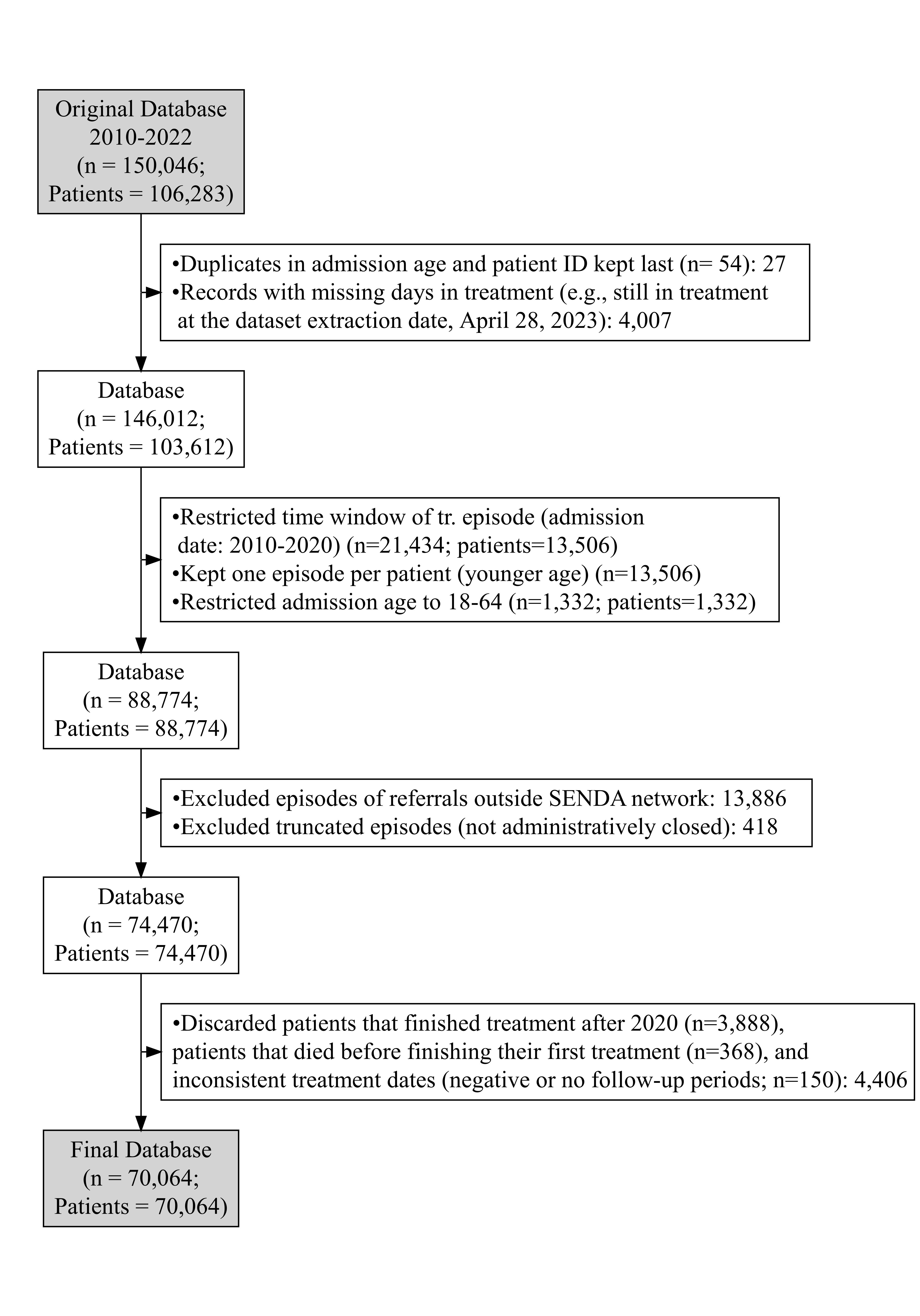
1.Number of cases before discarding duplicates in admission age and hash key: 150,046
1.Number of patients before discarding duplicates in admission age and hash key: 106,283
Records with unavailable missing days in treatment (eg., currently in treatment): 4007
Records with negative days in treatment: 8
Records with more than 3 years in treatment: 1039
1.Number of cases after discarding duplicates in admission age and hash key and validating days in treatment: 146,012
1.Number of patients after discarding duplicates in admission age and hash key and validating days in treatment: 103,612
1.Number of cases before discarding duplicates in admission age and hash key: 150,046
1.Number of patients before discarding duplicates in admission age and hash key: 106,283
Records with unavailable missing days in treatment (eg., currently in treatment): 4007
Records with negative days in treatment: 8
Records with more than 3 years in treatment: 1039
[1] 4007
[1] 4034
Si dije que descartaba quienes no completaban los ttos.
Discarded rows
[1] 4034
Discarded patients
[1] 2671Cohort Construction
Code
df0 <- SISTRAT23_c1_2010_2022_df_prev1q_sel2_surv
df1 <- df0 |>
filter(adm_date_rec2 >= "2010-01-01", adm_date_rec2 < "2021-01-01")
df2 <- df1 |>
arrange(hash_key, adm_date_rec2) |>
group_by(hash_key) |>
mutate(n_ttos = n(), tto = row_number(), post_ttos = as.integer(n_ttos > 1)) |>
slice_min(tto) |>
ungroup()
df3 <- df2 |>
filter(adm_age_rec2 >= 18, adm_age_rec2 < 65)

df2 |>
filter(adm_age_rec2 >= 65) |> count(!is.na(death_date))

warning("Muere el 18.5% de los atendidos >64")
Warning: Muere el 18.5% de los atendidos >64Code
audit <- data.frame(
step = c("inicio", "ventana temporal", "primer tratamiento", "edad 18-64"),
cases = c(nrow(df0), nrow(df1), nrow(df2), nrow(df3)),
patients = c(
nrow(distinct(df0, hash_key)),
nrow(distinct(df1, hash_key)),
nrow(distinct(df2, hash_key)),
nrow(distinct(df3, hash_key))
)
)
audit
# A tibble: 2 × 2
`!is.na(death_date)` n
<lgl> <int>
1 FALSE 978
2 TRUE 222
step cases patients
1 inicio 146014 103612
2 ventana temporal 124578 90106
3 primer tratamiento 90106 90106
4 edad 18-64 88774 88774Exclude Invalid Treatment Compliance
Code
days_years  <- 365.2425
censor_date <- as.Date("2020-12-31")

df4a_0 <- SISTRAT23_c1_2010_2022_df_prev1q_sel3a_surv
df4a_1 <- df4a_0 |>
  filter(
  !is.na(tr_compliance_rec3),
  tr_compliance_rec3 != "death",
  !grepl("truncated|currently|referral", tr_compliance_rec3)
  )
df4a_2 <- df4a_1 |>
  mutate(disch_age_rec = (dit_rec6 / days_years) + adm_age_rec2)
df4a_3 <- df4a_2 |>
  mutate(
  timesurv = case_when(
  status == 1 ~ lubridate::time_length(interval(adm_date_rec2, death_date), unit = "year"),
  status == 0 ~ lubridate::time_length(interval(adm_date_rec2, censor_date), unit = "year"),
  TRUE ~ NA_real_
  ),
  death_date_rec = case_when(
  status == 1 ~ death_date,
  status == 0 ~ censor_date,
  TRUE ~ as.Date(NA)
  ),
  death_age_rec = as.integer(timesurv + adm_age_rec2)
  )

SISTRAT23_c1_2010_2022_df_prev1q_sel4a_surv_rev <- df4a_3

cat("#_#_#_#_#_\nAudit table for 4a\n#_#_#_#_\n")
audit_4a <- data.frame(
step = c(
"start (3a)",
"exclude invalid tr. compliance",
"add discharge age",
"derive survival/death vars"
),
n = c(
nrow(df4a_0),
nrow(df4a_1),
nrow(df4a_2),
nrow(df4a_3)
),
patients = c(
nrow(distinct(df4a_0, hash_key)),
nrow(distinct(df4a_1, hash_key)),
nrow(distinct(df4a_2, hash_key)),
nrow(distinct(df4a_3, hash_key))
)
)
audit_4a
#_#_#_#_#_
Audit table for 4a
#_#_#_#_
step n patients
1 start (3a) 88774 88774
2 exclude invalid tr. compliance 74470 74470
3 add discharge age 74470 74470
4 derive survival/death vars 74470 74470Alternative Processing Path
Code
SISTRAT23_c1_2010_2022_df_prev1q_sel2_POST<-SISTRAT23_c1_2010_2022_df_prev1q_sel|>
tidytable::filter(adm_date_rec2>="2010-01-01", adm_date_rec2<"2020-12-31")|>
tidytable::arrange(hash_key, adm_age_rec2)|>
tidytable::filter(adm_date_rec2>="2010-01-01", adm_date_rec2<"2020-12-31")|>
tidytable::group_by(hash_key) |>
tidytable::mutate(tto= tidytable::row_number())|>
tidytable::slice_min(tto)|>
tidytable::ungroup()|>
tidytable::filter(adm_age_rec2>=18, adm_age_rec2<65)|>
tidytable::mutate(post_ttos=ifelse(tto>1, 1, 0))|>
(\(df) {
nrow(df)->>before_disc_dup_hash_age_adm_nrow_POST
cat(paste0("1.Number of cases before discarding duplicates in admission age and hash key: ", formatC(nrow(df), big.mark=",")),"\n")
cat(paste0("1.Number of patients before discarding duplicates in admission age and hash key: ", formatC(nrow(distinct(df, hash_key)), big.mark=",")),"\n")
mutate(df, years_in_tr= time_length(interval(adm_date_rec2, disch_date_rec6), unit="year")) |> filter(is.na(years_in_tr))->>alt_proc_miss_day_tr_curr_in;
cat(paste0("Records with unavailable missing days in treatment (eg., currently in treatment): ", nrow(alt_proc_miss_day_tr_curr_in), "\n"));
mutate(df, years_in_tr= time_length(interval(adm_date_rec2, disch_date_rec6), unit="year"))|> filter(years_in_tr<0) ->> alt_proc_neg_dit
cat(paste0("Records with negative days in treatment: ",nrow(alt_proc_neg_dit), "\n")) ;
mutate(df, years_in_tr= time_length(interval(adm_date_rec2, disch_date_rec6), unit="year"))|> filter(years_in_tr>3) ->> alt_proc_more3yr;
cat(paste0("Records with more than 3 years in treatment: ", nrow(alt_proc_more3yr), "\n"))
df
})()|>
mutate(years_in_tr= time_length(interval(adm_date_rec2, disch_date_rec6), unit="year"))|>
filter(!is.na(years_in_tr)|years_in_tr>=0|years_in_tr<=3)|>
group_by(hash_key, adm_age_rec2)|>
slice_max(dit_rec6)|>
ungroup()|>
(\(df) {
nrow(df)->>after_disc_dup_hash_age_adm_nrow_POST
cat(paste0("1.Number of cases after discarding duplicates in admission age and hash key and validating days in treatment: ", formatC(nrow(df), big.mark=",")),"\n")
cat(paste0("1.Number of patients after discarding duplicates in admission age and hash key and validating days in treatment: ", formatC(nrow(distinct(df, hash_key)), big.mark=",")),"\n")
df
})()

nrow(SISTRAT23_c1_2010_2022_df_prev1q_sel3a_surv)==nrow(SISTRAT23_c1_2010_2022_df_prev1q_sel2_POST)
identical(SISTRAT23_c1_2010_2022_df_prev1q_sel3a_surv,
SISTRAT23_c1_2010_2022_df_prev1q_sel2_POST)

warning("Se queda con la misma cantidad de pacientes, pero no son los mismos episodios\n")
Warning: Se queda con la misma cantidad de pacientes, pero no son los mismos episodiosCode
SISTRAT23_c1_2010_2022_df_prev1q_sel2_POST_surv<-
SISTRAT23_c1_2010_2022_df_prev1q_sel2_POST |>
tidytable::left_join(mortality[,c("hashkey", "death_date")], by=c("hash_key"="hashkey"), multiple="first") |>
tidytable::mutate(status=ifelse(is.na(death_date), 0, 1))

cat("\n#_#_#_#_#_\nAhora hacemos el proceso: Discarded ongoing treatments (truncated, death or currently in treatment, o referrals to teratments outside SENDA network).\n#_#_#_#_#_\n")
days_years<- 365.2425
SISTRAT23_c1_2010_2022_df_prev1q_sel4a_POST_surv<-
SISTRAT23_c1_2010_2022_df_prev1q_sel2_POST_surv|>
(\(df) {
nrow(df)->>df4a_nrow_pre_POST
cat(paste0("Discarded (death, no tr. compliance), cases(4a): ", formatC(nrow(tidytable::filter(df, is.na(tr_compliance_rec3) | tr_compliance_rec3=="death"|grepl("truncated|currently|referral", tr_compliance_rec3))), big.mark=",")),"\n")
cat(paste0("Discarded (death, no tr. compliance), patients(4a): ", formatC(nrow(distinct(tidytable::filter(df, is.na(tr_compliance_rec3) | tr_compliance_rec3=="death"|grepl("truncated|currently|referral", tr_compliance_rec3)), hash_key)), big.mark=",")),"\n")
df
})()|>
tidytable::filter(!is.na(tr_compliance_rec3) & tr_compliance_rec3!="death" & !grepl("truncated|currently|referral", tr_compliance_rec3))|>
tidytable::mutate(disch_age_rec= (dit_rec6/365.241)+adm_age_rec2)|>
tidytable::mutate(timesurv= tidytable::case_when(
status==1~ time_length(interval(adm_date_rec2, death_date), unit="year"),
status==0~ time_length(interval(adm_date_rec2, as.Date("2020-12-31")), unit="year")))|>
tidytable::mutate(death_date_rec= tidytable::case_when(
status==1~ death_date,
status==0~ as.Date("2020-12-31")))|>
tidytable::mutate(death_age_rec= as.integer(timesurv+adm_age_rec2))|>
(\(df) {
cat(paste0("4a.Number of cases: ", formatC(nrow(df), big.mark=",")),"\n")
cat(paste0("4a.Number of patients: ", formatC(nrow(distinct(df, hash_key)), big.mark=",")),"\n")
nrow(df) ->>df4a_nrow_post_POST
df
})()
1.Number of cases before discarding duplicates in admission age and hash key: 88,929
1.Number of patients before discarding duplicates in admission age and hash key: 88,929
Records with unavailable missing days in treatment (eg., currently in treatment): 155
Records with negative days in treatment: 7
Records with more than 3 years in treatment: 690
1.Number of cases after discarding duplicates in admission age and hash key and validating days in treatment: 88,774
1.Number of patients after discarding duplicates in admission age and hash key and validating days in treatment: 88,774
[1] TRUE
[1] FALSE
#_#_#_#_#_
Ahora hacemos el proceso: Discarded ongoing treatments (truncated, death or currently in treatment, o referrals to teratments outside SENDA network).
#_#_#_#_#_
Discarded (death, no tr. compliance), cases(4a): 14,311
Discarded (death, no tr. compliance), patients(4a): 14,311
4a.Number of cases: 74,464
4a.Number of patients: 74,463 Final Dataset Summary
Code
cat("Discarded records:\n")
df4a_nrow_pre_POST-df4a_nrow_post_POST
invisible("Ojo, hay más casos que pacientes (+1)\n")

clean_df |>
filter( rn %in% alt_proc_miss_day_tr_curr_in$rn) |> nrow()

invisible("Ninguno persiste de sin días en tto por ttos en curso\n")

clean_df |>
filter( rn %in% alt_proc_neg_dit$rn) |> nrow()
invisible("Ya ninguno persiste de los días de tto negativos\n")

clean_df |>
filter( rn %in% alt_proc_more3yr $rn) |> nrow()
invisible("278 con mpas de 3 años persisten en la base final\n")
Discarded records:
[1] 14311
[1] 0
[1] 0
[1] 278Flowchart
Code
neg_tr_d<- table(as.numeric(with(SISTRAT23_c1_2010_2022_df_prev1q_sel4a_surv,
difftime(death_date_rec, disch_date_rec6, unit="days"))/ 365.25)<0)[[2]]
over3yrs<-
table(as.numeric(with(SISTRAT23_c1_2010_2022_df_prev1q_sel4a_surv,
difftime(disch_date_rec6, adm_date_rec2, unit="days"))/ 365.25)>3)[[2]]

cat("#_#_#_#_#_\ncon las3 anteriores hago este:\n#_#_#_#_")

disch_after_cens_death

SISTRAT23_c1_2010_2022_df_prev1q_sel4a_surv |>
dplyr::filter(disch_date_rec6 >= death_date_rec) |>
dplyr::filter(death_date_rec=="2020-12-31", is.na(death_date)) |> nrow()

SISTRAT23_c1_2010_2022_df_prev1q_sel4a_surv |>
dplyr::filter(disch_date_rec6 >= death_date_rec) |>
dplyr::filter(!is.na(death_date)) |> nrow()

SISTRAT23_c1_2010_2022_df_prev1q_sel4a_surv |>
dplyr::filter(adm_date_rec2 >= disch_date_rec6) |> nrow()

invisible("No me gustó este criterio, pero lo ocupé. Sin querer eliminé 10 muertos\n")

SISTRAT23_c1_2010_2022_df_prev1q_sel4a_surv |>
dplyr::filter(adm_date_rec2 >= disch_date_rec6) |>
dplyr::filter(!is.na(death_date)) |> nrow()

368+3888+150

invisible("Qué pasa si aplicamos el filtro corregido para aprovechar los 0\nDIT en el análisis de sensibilidad\n")

SISTRAT23_c1_2010_2022_df_prev1q_sel4c_surv|>
mutate(disch_date_corr= as.Date(disch_date_corr2))|>
(\(df) {
cat("Before discarding missing or discharge dates\n")
print(nrow(df))
df
})()  |>
filter(#!is.na(disch_date_corr),
#!is.na(death_date_rec),
#disch_date_corr <= death_date_rec,
adm_date_rec2  >= disch_date_corr) |> nrow()

invisible("En la base de sensibilidad en que imputo con la mediana,\n202 tienen fecha de ingreso posterior o igual a la de egreso, y los elimino\n")

invisible("Pacientes con fechas de ingresos iguales o mayores a la de egreso: 150\n")
invisible("Pacientes en primer tratamiento que terminaron posterior al 2020-12-31, los elimino: 3888.\n")
invisible("Pacientes mueren antes de terminar el primer tto., los elimino: 368\n")

nrow(clean_df)
#_#_#_#_#_
con las3 anteriores hago este:
#_#_#_#_[1] 4256
[1] 3888
[1] 368
[1] 150
[1] 10
[1] 4406
Before discarding missing or discharge dates
[1] 88774
[1] 202
[1] 70064Code
gr<-
DiagrammeR::grViz("
digraph flowchart {
graph [layout = dot, rankdir = TB, nodesep = 0.2, ranksep = 0.3]
# General node styling
node [fontname = Times, shape = rectangle, fontsize = 17, style = filled, fillcolor = transparent]
# Main flow nodes
original [label = 'Original Database\\n2010-2022\\n(n = 150,046;\\nPatients = 106,283)', fillcolor = lightgray]
c1_dataset [label = 'Database\\n(n = 146,012;\\nPatients = 103,612)']
after_discard [label = 'Database\\n(n = 88,774;\\nPatients = 88,774)']
after_discard2 [label = 'Database\\n(n = 74,470;\\nPatients = 74,470)']
final_dataset [label = 'Final Database\\n(n = 70,064;\\nPatients = 70,064)', fillcolor = lightgray]
# Discard nodes (aligned between main flow steps)
discard_referrals [label = '•Duplicates in admission age and patient ID kept last (n= 54): 27\\l•Records with missing days in treatment (e.g., still in treatment\\l at the dataset extraction date, April 28, 2023): 4,007\\l']
discard_duplicates [label = '•Restricted time window of tr. episode (admission\\l date: 2010-2020) (n=21,434; patients=13,506)\\l•Kept one episode per patient (younger age) (n=13,506)\\l•Restricted admission age to 18-64 (n=1,332; patients=1,332)\\l'
]
discard_single [label = '•Excluded episodes of referrals outside SENDA network: 13,886\\l•Excluded truncated episodes (not administratively closed): 418\\l'
] // •Discarded (death, no tr. compliance): 14,304
discard_single2 [label = '•Discarded patients that finished treatment after 2020 (n=3,888),\\l patients that died before finishing their first treatment (n=368), and \\linconsistent treatment dates (negative or no follow-up periods; n=150): 4,406\\l']
# Invisible vertices for middle line
v1 [shape = point, width = 0, style = invis]
v2 [shape = point, width = 0, style = invis]
v3 [shape = point, width = 0, style = invis]
v4 [shape = point, width = 0, style = invis]
# Main flow edges (vertical line)
original -> v1 [arrowhead = none]
v1 -> c1_dataset
c1_dataset -> v2 [arrowhead = none]
v2 -> after_discard
after_discard ->v3 [arrowhead = none]
v3 -> after_discard2
after_discard2 -> v4 [arrowhead = none]
v4 -> final_dataset
# Discard connections (from the middle line)
v1 -> discard_referrals
v2 -> discard_duplicates
v3 -> discard_single
v4 -> discard_single2
# Alignment
{ rank = same; discard_referrals; v1 }
{ rank = same; discard_duplicates; v2 }
{ rank = same; discard_single; v3 }
{ rank = same; discard_single2; v4 }
}
", width = 1100, height = 1550)
base <- gsub("/cons","", getwd())
fig_dir <- file.path(base, "cons/_figs")
dir.create(fig_dir, recursive = TRUE, showWarnings = FALSE)
html_file <- file.path(fig_dir, "_mortality_flowchart_corr.html")
png_file <- file.path(fig_dir, "_mortality_flowchart_corr.png")
# Guarda el widget
htmlwidgets::saveWidget(gr, html_file, selfcontained = TRUE)
# Captura grande y nítida
webshot::webshot(
url = html_file,
file = png_file,
vwidth = 1100,
vheight = 1550,
zoom = 4, # 1100*4 = 4400 px de ancho aprox
expand = 20
)
Code
png_file[1] "G:/My Drive/Alvacast/SISTRAT 2023/cons/_figs/_mortality_flowchart_corr.png"Corrected main analysis
5-Year Bins
Code
invisible("Para comparar si hay alguna categoría muy chica en muestra, e inestable\n")

mltper_5x1 <- try(rio::import(paste0(base_path, "mltper_5x1.txt")))
fltper_5x1 <- try(rio::import(paste0(base_path, "fltper_5x1.txt")))
mltper_5x1_filt<-mltper_5x1[between(mltper_5x1$Year,2010,2020),]
fltper_5x1_filt<-fltper_5x1[between(fltper_5x1$Year,2010,2020),]
mltper_5x1_filt$age_rec <- as.numeric(mltper_5x1_filt$Age)
Warning: NAs introducidos por coerciónCode
fltper_5x1_filt$age_rec <- as.numeric(fltper_5x1_filt$Age)Warning: NAs introducidos por coerciónCode
mltper_5x1_filt$sex <- "male"
fltper_5x1_filt$sex <- "female"
cons_rate_sex_5x1<-
rbind.data.frame(mltper_5x1_filt, fltper_5x1_filt)[,c("Year","Age","sex", "lx","qx","mx")]
cons_rate_sex_5x1$lambda_p <- -log( 1 - cons_rate_sex_5x1$qx ) / 365.241
cons_rate_sex_5x1<-cons_rate_sex_5x1[which(cons_rate_sex_5x1$Age!="110+"),]

mx_national_raw <- cons_rate_sex_5x1
mx_national_clean <- mx_national_raw |>
  dplyr::mutate(
  agegroup = dplyr::case_when(
  Age == "0"   ~ 0,
  Age == "1-4" ~ 1,
  TRUE         ~ as.numeric(stringr::str_extract(Age, "^[0-9]+"))
  ),
  sex = stringr::str_to_title(sex),
  year = as.integer(Year)
  ) |>
  dplyr::select(year, sex, agegroup, mx) |>
  dplyr::distinct(year, sex, agegroup, .keep_all = TRUE) |>
  dplyr::arrange(year, sex, agegroup)

std_age_breaks <- c(0, 1, seq(5, 85, by = 5))
age_breaks <- sort(unique(mx_national_clean$agegroup))
age_breaks <- age_breaks[age_breaks >= 15]

c_SISTRAT_std_bins <- lexpand(
  clean_df,
  status = status,
  birth = birth_date_rec,
  exit = death_date_rec,
  entry = disch_date_rec6,
  breaks = list(
  per = seq(2010, 2021, by = 1),
  age = age_breaks
  ),
  aggre = list(year = per,
    agegroup = age,
    sex = sex_rec)
)

cat("Agegroups:\n")
sort(unique(c_SISTRAT_std_bins$agegroup))
Agegroups:
[1] 15 20 25 30 35 40 45 50 55 60 65 70 75SMR with 5-Year Bins
Code
sir_final_std <- sir(
  coh.data = c_SISTRAT_std_bins,
  coh.obs = 'from0to1',
  coh.pyrs = 'pyrs',
  ref.data = mx_national_clean,
  ref.rate = 'mx',
  adjust = c('agegroup', 'year', 'sex')
)
print(sir_final_std)

cat("Check differences in age-sex-year strata\n")
keys_coh <- unique(c_SISTRAT_std_bins[, c("year","sex","agegroup")])
keys_ref <- unique(mx_national_clean[, c("year","sex","agegroup")])
stopifnot(
  nrow(dplyr::anti_join(keys_coh, keys_ref, by=c("year","sex","agegroup")))==0
)

sir_ci_phi_improved( sir_final_std, extract_phi(c_SISTRAT_std_bins)) |>
  dplyr::mutate(print= sprintf("%.2f (%.2f–%.2f)",
  SIR,
  CI_low,
  CI_high)) |>
  data.table::data.table()
SIR (adjusted by agegroup, year, sex) with 95% confidence intervals (profile)
Total sir: 3.65 (3.52-3.78)
Total observed: 2996
Total expected: 820.46
Total person-years: 353826
observed expected pyrs sir sir.lo sir.hi p_value
<num> <num> <num> <num> <num> <num> <num>
1: 2996 820.46 353826 3.65 3.52 3.78 0
Check differences in age-sex-year strata
SIR CI_low CI_high phi_used print
<num> <num> <num> <num> <char>
1: 3.651626 3.519707 3.788489 1.05589 3.65 (3.52–3.79)DSR with 5-Year Bins
Code
proy_ine_com_2010_2020_corr<-
rio::import("https://www.ine.gob.cl/docs/default-source/proyecciones-de-poblacion/cuadros-estadisticos/base-2017/ine_estimaciones-y-proyecciones-2002-2035_base-2017_comunas0381d25bc2224f51b9770a705a434b74.csv?sfvrsn=b6e930a7_3&download=true")|>
  tidyr::pivot_longer(cols = dplyr::starts_with("Poblacion"),
  names_to = "anio",
  values_to = "poblacion")|>
  dplyr::mutate(anio= gsub("Poblacion ","",anio), anio=as.numeric(anio))|>
  dplyr::filter(anio>=2010 & anio<=2020)|>
  dplyr::mutate(agegroup = floor(Edad / 5) * 5) |>
  dplyr::filter(agegroup >= 15 & agegroup <= 75)|>
  dplyr::mutate(sex_rec= ifelse(`Sexo (1=Hombre 2=Mujer)`==2,"female","male"))|>
  group_by(anio, agegroup, sex_rec)|>
  summarise(pop=sum(poblacion, na.rm=T))|>
  ungroup()|>
  rename("year"="anio")
`summarise()` has grouped output by 'anio', 'agegroup'. You can override using
the `.groups` argument.Code
weights_corr <- proy_ine_com_2010_2020_corr |>
  dplyr::group_by(year, sex_rec, agegroup) |>
  dplyr::summarise(pop = sum(pop), .groups = "drop") |>
  dplyr::mutate(weights = pop / sum(pop)) |>
  dplyr::rename(sex = sex_rec) |>
  dplyr::select(year, sex, agegroup, weights)|>
  dplyr::mutate(sex = stringr::str_to_title(sex))

weights_corr <- data.table::as.data.table(weights_corr)[
  , .(year        = as.integer(year),
  agegroup    = as.integer(agegroup),
  sex         = factor(sex, levels = c("Male","Female")),
  weights     = as.numeric(weights))
]

proy_base <- proy_ine_com_2010_2020_corr |>
  dplyr::mutate(
    year = base::as.integer(year),
    agegroup = base::as.numeric(agegroup),
    sex = stringr::str_to_title(sex_rec)   # "Male"/"Female"
  )
w_year <- proy_base |>
  dplyr::summarise(pop = base::sum(pop), .by = year) |>
  dplyr::mutate(w = pop/base::sum(pop)) |>
  {\(d) stats::setNames(d$w, d$year)}()
w_sex <- proy_base |>
  dplyr::summarise(pop = base::sum(pop), .by = sex) |>
  dplyr::mutate(w = pop/base::sum(pop)) |>
  {\(d) stats::setNames(d$w, d$sex)}()


### Constructing weights  ======================

# Named weights vector in the order of levels you pass
make_w_named <- function(df, var, lev) {
  tmp <- df |>
    dplyr::summarise(pop = base::sum(pop), .by = dplyr::all_of(var)) |>
    dplyr::mutate(w = pop / base::sum(pop))

  tmp <- tmp[base::match(lev, tmp[[var]]), , drop = FALSE]
  stats::setNames(tmp$w, tmp[[var]])
}
#________________
# Cohort: real levels
#________________
lev_year <- 2010:2020
lev_sex  <- c("Male", "Female")

#________________
# Make weights
#________________
proy_for_w <- proy_base |>
  dplyr::filter(year %in% lev_year)
w_year <- make_w_named(proy_for_w, "year", lev_year)
w_sex  <- make_w_named(proy_for_w, "sex",  lev_sex)

### Constructing weights  ======================
#________________
# Cohort: real levels
#________________
# For 5 -year bins
lev_age_5y  <- base::sort(base::unique(c_SISTRAT_std_bins$agegroup))
lev_year_5y <- base::sort(base::unique(c_SISTRAT_std_bins$year))
proy_5y <- proy_base |>
  dplyr::filter(year %in% lev_year_5y, agegroup %in% lev_age_5y) |>
  dplyr::summarise(pop = base::sum(pop), .by = c(year, agegroup))  # colapsa sex
#________________
# Make weights
#________________
# For 5 -year bins
w_year_5y <- make_w_named(proy_5y, "year", lev_year_5y)
w_age_5y  <- make_w_named(proy_5y, "agegroup", lev_age_5y)
Code
dsr_tot <- popEpi::rate(
data    = c_SISTRAT_std_bins,
obs     = "from0to1",
pyrs    = "pyrs",
adjust  = c("year","sex","agegroup"),
weights = weights_corr
)
dsr_tot$rate_1k <- dsr_tot$rate * 1e3

DSR_1k_corr_corr <- mapply(
dsr_format_corr,
dsr_tot$rate.adj,
dsr_tot$SE.rate.adj,
MoreArgs = list(
phi    = max(1,  extract_phi_dir(c_SISTRAT_std_bins)),
factor = 1e3,
digits = 6,
conf   = 0.95))
DSR_1k_corr_corr
[1] "10.638095 (8.637565–13.101965)"By age
Code
# 5y attained-age (15,20,...,75) -> old bins (18,30,45,60)
to_old_agegroup <- function(age5) {
  dplyr::case_when(
    age5 < 30 ~ 18,
    age5 < 45 ~ 30,
    age5 < 60 ~ 45,
    TRUE      ~ 60
  )
}

message("#_#_#_#_#_\n Transform to 15-year bins \n#_#_#_#_#_\n")
#_#_#_#_#_
Transform to 15-year bins
#_#_#_#_#_Code
c_SISTRAT_std_old <- c_SISTRAT_std_bins |>
  dplyr::mutate(agegroup_old = to_old_agegroup(agegroup)) |>
  dplyr::group_by(year, sex, agegroup_old) |>
  dplyr::summarise(
    pyrs     = base::sum(pyrs),
    from0to1 = base::sum(from0to1),
    .groups  = "drop"
  )
Code
phi_df_age_old <- extract_phi_by_age(c_SISTRAT_std_old |> dplyr::rename(agegroup = agegroup_old))

dsr_age_old <- popEpi::rate(
  data    = c_SISTRAT_std_old,
  obs     = "from0to1",
  pyrs    = "pyrs",
  print   = "agegroup_old",
  adjust  = c("year","sex"),
  weights = list(year = w_year, sex = w_sex)
)

phi_vec_age_old <- base::pmax(1, phi_df_age_old$phi[match(dsr_age_old$agegroup_old, phi_df_age_old$agegroup)])

# dplyr::select(dsr_age_old, rate, rate.lo, rate.hi)|>
#   mutate_if(is.numeric, ~sprintf("%1.1f",.*1e3))

dsr_age_old<- cbind.data.frame(dplyr::as_tibble(dsr_age_old),phi= phi_vec_age_old)

DSR_1k_corr_agegr_corr <- mapply(
  dsr_format_corr,
  dsr_age_old$rate.adj,
  dsr_age_old$SE.rate.adj,
  dsr_age_old$phi,
  MoreArgs = list(factor = 1e3, digits = 6, conf = .95)
)

format_interval <- function(s) {
  # Encuentra todas las coincidencias de números decimales
  m <- gregexpr("[0-9]+\\.[0-9]+", s)
  regmatches(s, m) <- lapply(regmatches(s, m), function(nums) {
    formatC(as.numeric(nums), format = "f", digits = 1)
  })
  s
}
#
# cat("\n#_#_#_#_#_#_#_\nResults of DSRs by age\n#_#_#_#_#_#_#_\n")
# data.table::data.table(as.vector(sapply(DSR_1k_corr_agegr_corr,
#                                         format_interval)))
Code
c_SISTRAT_std_bins_wold <- c_SISTRAT_std_bins |>
  dplyr::mutate(agegroup_old = to_old_agegroup(agegroup))

smr_age_old <-
popEpi::sir(c_SISTRAT_std_bins_wold, coh.obs = 'from0to1',
                        coh.pyrs = 'pyrs',
                        ref.data = mx_national_clean,
                        ref.rate = mx,
                        print = c("agegroup_old"),
                        adjust = c("year", "sex", "agegroup"), #2025-12-16: the original still adjusts for agegroup
                        test.type = "homogeneity",
                        conf.type = "wald", #conf.type = "wald" usa la aproximación normal de Poisson (la misma lógica que explicamos antes).
                        conf.level = 0.95, EAR = T)
smr_age_old
smr_age_old_tbl <- cbind.data.frame(dplyr::as_tibble(smr_age_old), phi=phi_vec_age_old)
SIR (adjusted by year, sex, agegroup) with 95% confidence intervals (wald)
Test for homogeneity: p < 0.001
Total sir: 3.65 (3.52-3.78)
Total observed: 2996
Total expected: 820.46
Total person-years: 353826
Clave <agegroup_old>
agegroup_old observed expected pyrs sir sir.lo sir.hi p_value EAR
<num> <num> <num> <num> <num> <num> <num> <num> <num>
1: 18 224 69.63 77124.89 3.22 2.82 3.67 0 2.002
2: 30 1070 270.87 183190.97 3.95 3.72 4.19 0 4.362
3: 45 1343 341.29 82118.63 3.94 3.73 4.15 0 12.198
4: 60 359 138.68 11391.48 2.59 2.33 2.87 0 19.341By sex
Code
phi_sex_df  <- extract_phi_by_sex(c_SISTRAT_std_bins)

dsr_by_sex <- popEpi::rate(
  data    = c_SISTRAT_std_bins,
  obs     = "from0to1",
  pyrs    = "pyrs",
  print   = "sex",
  adjust  = c("year","agegroup"),
  weights = list(year = w_year_5y, agegroup = w_age_5y)
)

# dplyr::select(dsr_by_sex, rate, rate.lo, rate.hi)|>
#   mutate_if(is.numeric, ~sprintf("%1.1f",.*1e3))
# #   rate rate.lo rate.hi
# # 1  8.9     8.6     9.3
# # 2  7.0     6.5     7.6

phi_sex_vec <- pmax(1, phi_sex_df$phi[match(dsr_by_sex$sex, phi_sex_df$sex)])
dsr_by_sex <- cbind.data.frame(dplyr::as_tibble(dsr_by_sex),phi= phi_sex_vec)

DSR_1k_corr_sex_corr <- mapply(
  dsr_format_corr,
  dsr_by_sex $rate.adj,
  dsr_by_sex $SE.rate.adj,
  phi     = pmax(1,phi_sex_vec)[match(dsr_by_sex$sex, phi_sex_df$sex)],
  MoreArgs = list(factor = 1e3, digits = 6, conf = .95)
)
# cat("\n#_#_#_#_#_#_#_\nResults of DSRs by sex\n#_#_#_#_#_#_#_\n")
# data.table::data.table(as.vector(sapply(DSR_1k_corr_sex_corr,
#                                         format_interval)))
# Male: 13.7 (9.5–19.9)
# Female:   7.9 (6.6–9.5)
Code
smr_sex_corr <- popEpi::sir(
  coh.data = c_SISTRAT_std_bins,
  coh.obs  = "from0to1",
  coh.pyrs = "pyrs",
  ref.data = mx_national_clean,
  ref.rate = "mx",
  print    = "sex",
  adjust   = c("year","sex","agegroup")  # <- 5y internal
)
smr_sex_corr

smr_sex_corr_tbl <- cbind.data.frame(dplyr::as_tibble(smr_sex_corr), phi=phi_sex_vec)

sir_ci_phi_improved( smr_sex_corr, smr_sex_corr_tbl$phi)|>
  dplyr::mutate(print= sprintf("%.2f (%.2f–%.2f)",
                               SIR,
                               CI_low,
                               CI_high)) |>
  data.table::data.table()
SIR (adjusted by year, sex, agegroup) with 95% confidence intervals (profile)
Test for homogeneity: p < 0.001
Total sir: 3.65 (3.52-3.78)
Total observed: 2996
Total expected: 820.46
Total person-years: 353826
Clave <sex>
sex observed expected pyrs sir sir.lo sir.hi p_value
<char> <num> <num> <num> <num> <num> <num> <num>
1: Female 600 107.72 85500.75 5.57 5.14 6.03 0
2: Male 2396 712.73 268325.23 3.36 3.23 3.50 0
SIR CI_low CI_high phi_used print
<num> <num> <num> <num> <char>
1: 5.569826 5.141519 6.033812 1 5.57 (5.14–6.03)
2: 3.361707 3.229760 3.499044 1 3.36 (3.23–3.50)Code
# -------------------------
# SEX (one row per sex)
# -------------------------
sir_sex_dt <- sir_ci_phi_improved(smr_sex_corr, smr_sex_corr_tbl$phi)
sir_sex_print <- fmt_interval(base::sprintf("%.2f (%.2f–%.2f)", sir_sex_dt$SIR, sir_sex_dt$CI_low, sir_sex_dt$CI_high))

sex_sir_map <- data.frame(
    Subgroup = base::as.character(smr_sex_corr_tbl$sex),
    SIR      = sir_sex_print,
    stringsAsFactors = FALSE
)

sex_subcol <- pick_col(dsr_by_sex, c("group","sex"))  # <-- THIS fixes your error

sex_dsr_vec <- fmt_interval(base::as.vector(base::sapply(DSR_1k_corr_sex_corr, format_interval)))

sex_cmr <- fmt_interval(base::paste0(
    base::sprintf("%1.1f", dsr_by_sex$rate*1e3),
    " (", base::sprintf("%1.1f", dsr_by_sex$rate.lo*1e3),
    "–", base::sprintf("%1.1f", dsr_by_sex$rate.hi*1e3), ")"
))

sex_tbl <- data.frame(
    Section = "Sex",
    Subgroup = base::as.character(dsr_by_sex[[sex_subcol]]),
    DSR_1k   = sex_dsr_vec,
    CMR_1k   = sex_cmr,
    Deaths   = dsr_by_sex$from0to1,
    `Person-years` = dsr_by_sex$pyrs,
    stringsAsFactors = FALSE
)

sex_tbl <- base::merge(sex_tbl, sex_sir_map, by = "Subgroup", all.x = TRUE)

# reorder
sex_tbl <- sex_tbl[, c("Section","Subgroup","SIR","DSR_1k","CMR_1k","Deaths","Person.years")]

# -------------------------
# AGE (one row per agegroup_old)
# -------------------------
sir_age_dt <- sir_ci_phi_improved(smr_age_old, smr_age_old_tbl$phi)
sir_age_print <- fmt_interval(base::sprintf("%.2f (%.2f–%.2f)", sir_age_dt$SIR, sir_age_dt$CI_low, sir_age_dt$CI_high))

age_subcol <- pick_col(smr_age_old_tbl, c("agegroup_old","agegroup"))
age_sir_map <- data.frame(
    Subgroup = base::as.character(smr_age_old_tbl[[age_subcol]]),
    SIR      = sir_age_print,
    stringsAsFactors = FALSE
)

age_dsr_vec <- fmt_interval(base::as.vector(base::sapply(DSR_1k_corr_agegr_corr, format_interval)))

age_cmr <- fmt_interval(base::paste0(
    base::sprintf("%1.1f", dsr_age_old$rate*1e3),
    " (", base::sprintf("%1.1f", dsr_age_old$rate.lo*1e3),
    "–", base::sprintf("%1.1f", dsr_age_old$rate.hi*1e3), ")"
))

age_tbl <- data.frame(
    Section = "Age group",
    Subgroup = base::as.character(dsr_age_old$agegroup_old),
    DSR_1k   = age_dsr_vec,
    CMR_1k   = age_cmr,
    Deaths   = dsr_age_old$from0to1,
    `Person-years` = dsr_age_old$pyrs,
    stringsAsFactors = FALSE
)

age_tbl <- base::merge(age_tbl, age_sir_map, by = "Subgroup", all.x = TRUE)
age_tbl <- age_tbl[, c("Section","Subgroup","SIR","DSR_1k","CMR_1k","Deaths","Person.years")]

# -------------------------
# OVERALL (single row)
# -------------------------
sir_overall_dt <- sir_ci_phi_improved(sir_final_std, extract_phi(c_SISTRAT_std_bins))
sir_overall_print <- fmt_interval(base::sprintf("%.2f (%.2f–%.2f)", sir_overall_dt$SIR, sir_overall_dt$CI_low, sir_overall_dt$CI_high))

cmr_overall <- fmt_interval(base::sprintf("%1.1f (%1.1f–%1.1f)",
                                      dsr_tot$rate*1e3, dsr_tot$rate.lo*1e3, dsr_tot$rate.hi*1e3
))
DSR_1k_corr_corr_1dec<-
    mapply(
        dsr_format_corr,                 # FUN
        dsr_tot$rate.adj,           # primer vector (rate)
        dsr_tot$SE.rate.adj,        # segundo vector (se)
        MoreArgs = list(            # argumentos fijos extra
            #phi    = extract_phi_dir(c_SISTRAT_std_bins),
            #opc. conservadora
            phi    = max(1,  extract_phi_dir(c_SISTRAT_std_bins)),
            factor = 1e3,
            digits = 1,
            conf   = 0.95))

overall_tbl <- data.frame(
    Section = "Overall",
    Subgroup = "All",
    SIR = sir_overall_print,
    DSR_1k = fmt_interval(DSR_1k_corr_corr_1dec),
    CMR_1k = cmr_overall,
    Deaths = sir_final_std$observed,
    `Person-years` = sir_final_std$pyrs,
    stringsAsFactors = FALSE
)

# -------------------------
# FINAL TABLE
# -------------------------
final_tbl <- base::rbind(overall_tbl, sex_tbl, age_tbl)

# format PY like your output
final_tbl$`Person.years` <- base::formatC(final_tbl$`Person.years`, format="f", digits=0, big.mark=",")
final_tbl$`Deaths` <- base::formatC(final_tbl$`Deaths`, format="f", digits=0, big.mark=",")

knitr::kable(
    final_tbl,
    caption = "SMR (with overdispersion adjustment) and DSR/CMR per 1,000 person-years.",
    align = c("l","l","l","l","l","r","r")
)| Section | Subgroup | SIR | DSR_1k | CMR_1k | Deaths | Person.years |
|---|---|---|---|---|---|---|
| Overall | All | 3.65 (3.52–3.79) | 10.6 (8.6–13.1) | 8.5 (8.2–8.8) | 2,996 | 353,826 |
| Sex | Female | 5.57 (5.14–6.03) | 7.9 (6.6–9.5) | 7.0 (6.5–7.6) | 600 | 85,501 |
| Sex | Male | 3.36 (3.23–3.50) | 13.7 (9.5–19.9) | 8.9 (8.6–9.3) | 2,396 | 268,325 |
| Age group | 18 | 3.22 (2.82–3.67) | 2.9 (2.4–3.4) | 2.9 (2.5–3.3) | 224 | 77,125 |
| Age group | 30 | 3.95 (3.69–4.23) | 5.7 (4.7–6.9) | 5.8 (5.5–6.2) | 1,070 | 183,191 |
| Age group | 45 | 3.94 (3.73–4.15) | 14.2 (12.9–15.7) | 16.4 (15.5–17.3) | 1,343 | 82,119 |
| Age group | 60 | 2.59 (2.33–2.87) | 46.8 (20.7–106.1) | 31.5 (28.4–34.9) | 359 | 11,391 |
Heterogeneity
Code
smr_sex_dat <- sir_ci_phi_improved( smr_sex_corr, smr_sex_corr_tbl$phi) |>
    dplyr::mutate(
        yi  = base::log(SIR),
        sei = se_log_from_ci(SIR, CI_low, CI_high, conf = 0.95)
    )

meta_smr_sex <- metafor::rma(
    yi = yi,
    sei = sei,
    method = "FE",
    data = smr_sex_dat
)

smr_age_dat <- sir_ci_phi_improved( smr_age_old, smr_age_old_tbl$phi) |>
    dplyr::mutate(
        yi  = base::log(SIR),
        sei = se_log_from_ci(SIR,CI_low, CI_high, conf = 0.95)
    )

meta_smr_age <- metafor::rma(
    yi = yi,
    sei = sei,
    method = "FE",
    data = smr_age_dat
)

dsr_sex_dat <- dsr_by_sex |>
    dplyr::mutate(sex = base::as.character(sex)) |>
    dplyr::mutate(
        yi  = base::log(rate.adj),
        sei = se_log_from_rate_se(rate.adj, SE.rate.adj, phi = phi)
    )

meta_dsr_sex <- metafor::rma(
    yi = yi,
    sei = sei,
    method = "FE",
    data = dsr_sex_dat
)

dsr_age_dat <- dsr_age_old |>
    dplyr::mutate(
        yi  = base::log(rate.adj),
        sei = se_log_from_rate_se(rate.adj, SE.rate.adj, phi = phi)
    )

meta_dsr_age <- metafor::rma(yi = yi, sei = sei, method = "FE", data = dsr_age_dat)


het_tbl <- base::rbind(
  het_row(meta_smr_sex, "SMR (SIR) by sex"),
  het_row(meta_smr_age, "SMR (SIR) by age group"),
  het_row(meta_dsr_sex, "DSR by sex"),
  het_row(meta_dsr_age, "DSR by age group")
)

knitr::kable(
  het_tbl,
  caption = "Heterogeneity tests (fixed-effect meta-analysis; Cochran’s Q and I²).",
  align = c("l","r","r","r","r")
)| Analysis | Q | df | p | I2 |
|---|---|---|---|---|
| SMR (SIR) by sex | 122.33 | 1 | 0.000 | 99.2 |
| SMR (SIR) by age group | 58.65 | 3 | 0.000 | 94.9 |
| DSR by sex | 6.84 | 1 | 0.009 | 85.4 |
| DSR by age group | 275.67 | 3 | 0.000 | 98.9 |
Code
dsr_sep <- strcapture("^\\s*([0-9.]+)\\s*\\(\\s*([0-9.]+)\\s*[–-]\\s*([0-9.]+)\\s*\\)\\s*$",
                      DSR_1k_corr_agegr_corr,
                      proto = list(estimate = numeric(),
                                   ci_low = numeric(),
                                   ci_high = numeric()))

age_labels <- c("18-29", "30-44", "45-59", "60+")

map_groups <- function(df, labels = age_labels) {
  df |>
    dplyr::mutate(
      group1 = ifelse(grepl("^Group", group1), labels[as.integer(sub("Group ", "", group1))], group1),
      group2 = ifelse(grepl("^Group", group2), labels[as.integer(sub("Group ", "", group2))], group2)
    )
}

tab_pairwise <- rbind.data.frame(
  tibble::tibble(
    group1     = "SMR",
    group2     = NA_character_,
    smr1       = NA_real_,
    smr2       = NA_real_,
    difference = NA_real_,
    ratio_1_over_2 = NA_real_,
    se_diff    = NA_real_,
    z          = NA_real_,
    p_unadj    = NA_real_,
    p_holm     = NA_real_
  ),
  pairwise_smr_test(
    smrs   = sir_ci_phi_improved( smr_age_old, smr_age_old_tbl$phi)[,1],
    lowers = sir_ci_phi_improved( smr_age_old, smr_age_old_tbl$phi)[,2],
    uppers = sir_ci_phi_improved( smr_age_old, smr_age_old_tbl$phi)[,3]
  ) |> map_groups(),
  tibble::tibble(
    group1     = "DSR",
    group2     = NA_character_,
    smr1       = NA_real_,
    smr2       = NA_real_,
    difference = NA_real_,
    ratio_1_over_2 = NA_real_,
    se_diff    = NA_real_,
    z          = NA_real_,
    p_unadj    = NA_real_,
    p_holm     = NA_real_
  ),
  pairwise_smr_test(
    smrs   = dsr_sep$estimate,
    lowers = dsr_sep$ci_low,
    uppers = dsr_sep$ci_high
  ) |> map_groups()
) |>
  dplyr::rename(estimate1 = smr1, estimate2 = smr2) |>
  dplyr::mutate(dplyr::across(c(se_diff, z), ~ round(., 2)))

knitr::kable(tab_pairwise, "markdown", caption = "Pairwise comparison, age groups")| group1 | group2 | estimate1 | estimate2 | difference | ratio_1_over_2 | se_diff | z | p_unadj | p_holm |
|---|---|---|---|---|---|---|---|---|---|
| SMR | NA | NA | NA | NA | NA | NA | NA | NA | NA |
| 18-29 | 30-44 | 3.217041 | 3.950297 | -0.7332560 | 0.8143795 | 0.08 | 2.73 | 0.0063795 | 0.0209779 |
| 18-29 | 45-59 | 3.217041 | 3.935117 | -0.7180760 | 0.8175211 | 0.07 | 2.79 | 0.0052445 | 0.0209779 |
| 18-29 | 60+ | 3.217041 | 2.588776 | 0.6282656 | 1.2426883 | 0.09 | 2.55 | 0.0107161 | 0.0214321 |
| 30-44 | 45-59 | 3.950297 | 3.935117 | 0.0151800 | 1.0038576 | 0.04 | 0.09 | 0.9304696 | 0.9304696 |
| 30-44 | 60+ | 3.950297 | 2.588776 | 1.3615216 | 1.5259327 | 0.06 | 6.69 | 0.0000000 | 0.0000000 |
| 45-59 | 60+ | 3.935117 | 2.588776 | 1.3463416 | 1.5200689 | 0.06 | 7.05 | 0.0000000 | 0.0000000 |
| DSR | NA | NA | NA | NA | NA | NA | NA | NA | NA |
| 18-29 | 30-44 | 2.883079 | 5.683480 | -2.8004010 | 0.5072735 | 0.13 | 5.04 | 0.0000005 | 0.0000014 |
| 18-29 | 45-59 | 2.883079 | 14.212263 | -11.3291840 | 0.2028585 | 0.10 | 15.32 | 0.0000000 | 0.0000000 |
| 18-29 | 60+ | 2.883079 | 46.833428 | -43.9503490 | 0.0615603 | 0.43 | 6.53 | 0.0000000 | 0.0000000 |
| 30-44 | 45-59 | 5.683480 | 14.212263 | -8.5287830 | 0.3998997 | 0.11 | 8.25 | 0.0000000 | 0.0000000 |
| 30-44 | 60+ | 5.683480 | 46.833428 | -41.1499480 | 0.1213552 | 0.43 | 4.92 | 0.0000009 | 0.0000018 |
| 45-59 | 60+ | 14.212263 | 46.833428 | -32.6211650 | 0.3034641 | 0.42 | 2.84 | 0.0045613 | 0.0045613 |
By strata
Code
clean_df2 <- clean_df |>
dplyr::mutate(
setting = dplyr::if_else(res_plan == 1, "Residential", "Ambulatory"),
setting = base::factor(setting, levels = c("Ambulatory","Residential")),
completed = base::as.character(tr_compliance_status),
completed = base::factor(completed, levels = c("Completed","Not completed")),
licit_illicit = base::as.character(prim_sub_licit),
licit_illicit = base::factor(licit_illicit, levels = c("licit","illicit")),
disch_age_cat = base::as.character(disch_age_cat),
disch_age_cat = base::factor(disch_age_cat, levels = c("18-29","30-44","45-59","60+")),
sex = stringr::str_to_title(base::as.character(sex_rec)),
sex = base::factor(sex, levels = c("Male","Female"))
)
c_SISTRAT_5y <- popEpi::lexpand(
data   = clean_df2,
status = status,
birth  = birth_date_rec,
entry  = disch_date_rec6,
exit   = death_date_rec,
breaks = list(
per = base::seq(2010, 2021, by = 1),
age = age_breaks
),
aggre = list(
year    = per,
agegroup= age,
sex     = sex,
setting      = setting,
completed    = completed,
licit_illicit= licit_illicit,
disch_age_cat= disch_age_cat
)
)

warning("disch_age_cat es edad al alta (baseline) → perfecto para “preservar
los grupos antiguos” aunque el Lexis use attained-age 5y internamente para el ajuste.")
Warning: disch_age_cat es edad al alta (baseline) → perfecto para “preservar
los grupos antiguos” aunque el Lexis use attained-age 5y internamente para el ajuste.Code
dsr_setting <- run_dsr_by(c_SISTRAT_5y, weights_corr, "setting")Warning: There was 1 warning in `dplyr::summarise()`.
ℹ In argument: `result = list(...)`.
ℹ In group 1: `setting = Ambulatory`.
Caused by warning:
! `cur_data_all()` was deprecated in dplyr 1.1.0.
ℹ Please use `pick()` instead.Code
dsr_completed <- run_dsr_by(c_SISTRAT_5y, weights_corr, "completed")
dsr_licit     <- run_dsr_by(c_SISTRAT_5y, weights_corr, "licit_illicit")
Code
tbl_all <- base::rbind(
  prep_dsr(dsr_setting,   "Setting"),
  prep_dsr(dsr_completed, "Completion"),
  prep_dsr(dsr_licit,     "Licit/illicit")#,  prep_dsr(dsr_age,       "Age group")
)

knitr::kable(
  tbl_all,
  caption = "Directly standardized rates (DSR) and crude mortality rates (CMR), per 1,000 person-years, across subgroups.",
  align = c("l","l","r","r","r","r","r","l","r","r","r","r")
)| Section | Group | Deaths | Person-years | DSR/1,000 | DSR L | DSR U | DSR/1,000 (95% CI) | CMR/1,000 | CMR L | CMR U | Phi |
|---|---|---|---|---|---|---|---|---|---|---|---|
| Setting | Ambulatory | 2488 | 302,963.3 | 10.54 | 8.24 | 13.49 | 10.54 (8.24–13.49) | 8.21 | 7.90 | 8.54 | 1.337 |
| Setting | Residential | 508 | 50,862.7 | 9.73 | 7.91 | 11.96 | 9.73 (7.91–11.96) | 9.99 | 9.16 | 10.90 | 1.271 |
| Completion | Completed | 671 | 83,248.2 | 7.66 | 5.90 | 9.94 | 7.66 (5.90–9.94) | 8.06 | 7.47 | 8.69 | 1.629 |
| Completion | Not completed | 2325 | 270,577.8 | 11.93 | 9.22 | 15.44 | 11.93 (9.22–15.44) | 8.59 | 8.25 | 8.95 | 1.443 |
| Licit/illicit | licit | 1742 | 107,780.2 | 12.82 | 10.89 | 15.09 | 12.82 (10.89–15.09) | 16.16 | 15.42 | 16.94 | 1.505 |
| Licit/illicit | illicit | 1254 | 246,045.8 | 8.78 | 5.74 | 13.44 | 8.78 (5.74–13.44) | 5.10 | 4.82 | 5.39 | 1.000 |
Code
smr_setting   <- run_smr_by(c_SISTRAT_5y, mx_national_clean, "setting")
smr_completed <- run_smr_by(c_SISTRAT_5y, mx_national_clean, "completed")
smr_licit     <- run_smr_by(c_SISTRAT_5y, mx_national_clean, "licit_illicit")
#smr_agecat    <- run_smr_by(c_SISTRAT_5y, mx_national_clean, "disch_age_cat")
smr_setting_phi <- smr_setting%>%
dplyr::left_join(dplyr::select(dsr_setting, group, phi), by = "group")%>%
sir_ci_phi_profile(phi = .$phi) |>
dplyr::mutate(print = sprintf(paste0("%.", 2, "f (%.", 2, "f–%.", 2, "f)"),
sir, sir.phi.lo, sir.phi.hi))
smr_completed_phi <- smr_completed%>%
dplyr::left_join(dplyr::select(dsr_completed, group, phi), by = "group")%>%
sir_ci_phi_profile(phi = .$phi) |>
dplyr::mutate(print = sprintf(paste0("%.", 2, "f (%.", 2, "f–%.", 2, "f)"),
sir, sir.phi.lo, sir.phi.hi))
smr_licit_phi <- smr_licit%>%
dplyr::left_join(dplyr::select(dsr_licit, group, phi), by = "group")%>%
sir_ci_phi_profile(phi = .$phi) |>
dplyr::mutate(print = sprintf(paste0("%.", 2, "f (%.", 2, "f–%.", 2, "f)"),
sir, sir.phi.lo, sir.phi.hi))
# smr_agecat_phi <- smr_agecat%>%
# dplyr::left_join(subset(run_dsr_by_agecat(c_SISTRAT_5y, w_year, w_sex), select=c("group","phi")),
# by = "group")%>%
# sir_ci_phi_profile(phi = .$phi) |>
# dplyr::mutate(print = sprintf(paste0("%.", 2, "f (%.", 2, "f–%.", 2, "f)"),
# sir, sir.phi.lo, sir.phi.hi))
Code
# Combine all tables into one with a "Category" column
smr_table <- bind_rows(
  smr_setting_phi %>% mutate(Category = "Setting") %>% dplyr::select(Category, Group = group, Observed = observed, Expected = expected, SMR = print),
  smr_completed_phi %>% mutate(Category = "Treatment Completion") %>% dplyr::select(Category, Group = group, Observed = observed, Expected = expected, SMR = print),
  smr_licit_phi %>% mutate(Category = "Primary Substance") %>% dplyr::select(Category, Group = group, Observed = observed, Expected = expected, SMR = print)#,
  # smr_agecat_phi %>% mutate(Category = "Age at Discharge") %>% select(Category, Group = group, Observed = observed, Expected = expected, SMR = print)
) %>%
  mutate(
    Category = ifelse(
      Category != lag(Category, default = ""),
      Category,
      ""
    )
  )

# Create kable
kable(
  smr_table,
  col.names = c("Category", "Group", "Observed", "Expected", "SMR (95% CI)"),
  align = c("l", "l", "r", "r", "r"),
  booktabs = TRUE,
  linesep = ""
) | Category | Group | Observed | Expected | SMR (95% CI) |
|---|---|---|---|---|
| Setting | Ambulatory | 2488 | 717.0084 | 3.47 (3.32–3.63) |
| Residential | 508 | 103.4480 | 4.91 (4.45–5.42) | |
| Treatment Completion | Completed | 671 | 245.0630 | 2.74 (2.49–3.02) |
| Not completed | 2325 | 575.3933 | 4.04 (3.85–4.24) | |
| Primary Substance | licit | 1742 | 379.3954 | 4.59 (4.33–4.86) |
| illicit | 1254 | 441.0610 | 2.84 (2.69–3.00) |
Heterogeneity
Code
# --- DSR: Treatment Setting ---
meta_dsr_setting <- dsr_setting |>
  dplyr::mutate(
    # Use phi if present, else 1
    phi_used = if("phi" %in% names(dsr_setting)) phi else 1,
    yi  = log(rate.adj),
    sei = (SE.rate.adj * sqrt(phi_used)) / rate.adj
  ) |>
  metafor::rma(yi = yi, sei = sei, method = "FE", data = _)

# --- SMR: Treatment Setting ---
meta_smr_setting <- smr_setting_phi |>
  dplyr::mutate(
    yi  = log(sir),
    # Calculate SE on log scale from the Phi-corrected CIs (averaging upper and lower)
    sei = 0.5 * ((log(sir.phi.hi) - log(sir))/1.96 + (log(sir) - log(sir.phi.lo))/1.96)
  ) |>
  metafor::rma(yi = yi, sei = sei, method = "FE", data = _)

# --- DSR: Compliance ---
meta_dsr_compl <- dsr_completed |>
  dplyr::mutate(
    phi_used = if("phi" %in% names(dsr_completed)) phi else 1,
    yi  = log(rate.adj),
    sei = (SE.rate.adj * sqrt(phi_used)) / rate.adj
  ) |>
  metafor::rma(yi = yi, sei = sei, method = "FE", data = _)

# --- SMR: Compliance ---
meta_smr_compl <- smr_completed_phi |>
  dplyr::mutate(
    yi  = log(sir),
    sei = 0.5 * ((log(sir.phi.hi) - log(sir))/1.96 + (log(sir) - log(sir.phi.lo))/1.96)
  ) |>
  metafor::rma(yi = yi, sei = sei, method = "FE", data = _)

# --- DSR: Licit/Illicit ---
meta_dsr_licit <- dsr_licit |>
  dplyr::mutate(
    phi_used = if("phi" %in% names(dsr_licit)) phi else 1,
    yi  = log(rate.adj),
    sei = (SE.rate.adj * sqrt(phi_used)) / rate.adj
  ) |>
  metafor::rma(yi = yi, sei = sei, method = "FE", data = _)

# --- SMR: Licit/Illicit ---
meta_smr_licit <- smr_licit_phi |>
  dplyr::mutate(
    yi  = log(sir),
    sei = 0.5 * ((log(sir.phi.hi) - log(sir))/1.96 + (log(sir) - log(sir.phi.lo))/1.96)
  ) |>
  metafor::rma(yi = yi, sei = sei, method = "FE", data = _)


het_tbl <- base::rbind(
  het_row_strata(meta_dsr_setting, "Setting",        "DSR"),
  het_row_strata(meta_smr_setting, "Setting",        "SMR"),
  het_row_strata(meta_dsr_compl,   "Compliance",     "DSR"),
  het_row_strata(meta_smr_compl,   "Compliance",     "SMR"),
  het_row_strata(meta_dsr_licit,   "Licit/Illicit",  "DSR"),
  het_row_strata(meta_smr_licit,   "Licit/Illicit",  "SMR")
)

knitr::kable(
  het_tbl,
  caption = "Heterogeneity tests (fixed-effect meta-analysis): Cochran’s Q and I² for subgroup contrasts.",
  align = c("l","l","r","r","r","r")
)| Contrast | Outcome | Q | df | p | I2 |
|---|---|---|---|---|---|
| Setting | DSR | 0.24 | 1 | 0.626 | 0.0 |
| Setting | SMR | 39.67 | 1 | 0.000 | 97.5 |
| Compliance | DSR | 5.62 | 1 | 0.018 | 82.2 |
| Compliance | SMR | 49.67 | 1 | 0.000 | 98.0 |
| Licit/Illicit | DSR | 2.65 | 1 | 0.104 | 62.2 |
| Licit/Illicit | SMR | 138.29 | 1 | 0.000 | 99.3 |
By causes
Code
years_keep    <- base::sort(base::unique(base::as.integer(c_SISTRAT_std_bins_wold$year)))
agegroups_keep<- base::sort(base::unique(base::as.integer(c_SISTRAT_std_bins_wold$agegroup)))

mx_national_by_cause <- build_mx_national_by_cause(
  deaths_nat_df = mortality_deduplicated,
  pop_df        = proy_ine_com_2010_2020_corr,
  years_keep    = years_keep,
  agegroups_keep= agegroups_keep,
  year_col  = "ano_def",
  sex_col   = "sexo",
  age_col   = "edad_cant",
  diag1_col = "diag1",
  diag2_col = "diag2",
  pop_sex_col = "sex_rec"
)

clean_df3<- left_join(clean_df2,
  dplyr::select(mortality_deduplicated,
  hashkey,
  diag1,
  diag2 ), by=c("hash_key"="hashkey"))
coh_cause <- build_cohort_by_cause(clean_df3, c_SISTRAT_5y)

smr_cause <- popEpi::sir(
  coh.data = coh_cause,
  coh.obs  = "from0to1",
  coh.pyrs = "pyrs",
  ref.data = mx_national_by_cause,
  ref.rate = "mx",
  print    = "cause_cat",
  adjust   = c("year","sex","agegroup","cause_cat")
  ) |>
  dplyr::as_tibble()
Could not solve profile-likelihood. Wald confidence intervals selected.Code
warning("In trasnport accidents, in fact were observed 162 and expected 77.5")Warning: In trasnport accidents, in fact were observed 162 and expected 77.5Code
mortality_deduplicated |>
  tidytable::mutate(
    icd = stringr::str_to_upper(as.character(diag1)),
    icd = stringr::str_replace_all(icd, "\\.", ""),
    icd3 = stringr::str_extract(icd, "^[A-Z][0-9]{2}"),
    cause_cat = assign_cause_cat_vec_corr(diag1, diag2)
  ) |>
  tidytable::summarise(
  n = .N,
  n_na = sum(is.na(cause_cat)),
  prop_na = mean(is.na(cause_cat))
  )

warning("From 2025-12-30, now there are no NAs")
Warning: From 2025-12-30, now there are no NAsCode
phi_global <- extract_phi_global(coh_cause, rhs_vars = c("year","sex","agegroup"))
phi_cause <- extract_phi_by(
    coh_cause,
    by = "cause_cat",
    rhs_vars = c("year","sex","agegroup"),
    min_events = 20,
    phi_fallback = phi_global
    )
Warning: There were 11 warnings in `dplyr::summarise()`.
The first warning was:
ℹ In argument: `result = list(...)`.
ℹ In group 1: `cause_cat = "Infectious & parasitic (A00–B99)"`.
Caused by warning:
! glm.fit: fitted rates numerically 0 occurred
ℹ Run `dplyr::last_dplyr_warnings()` to see the 10 remaining warnings.Code
dsr_cause <- run_dsr_by_cause(coh_cause, weights_corr, digits = 2)Warning: There were 11 warnings in `dplyr::summarise()`.
The first warning was:
ℹ In argument: `result = list(...)`.
ℹ In group 1: `cause_cat = "Infectious & parasitic (A00–B99)"`.
Caused by warning:
! glm.fit: fitted rates numerically 0 occurred
ℹ Run `dplyr::last_dplyr_warnings()` to see the 10 remaining warnings.# A tidytable: 1 × 3
n n_na prop_na
<int> <int> <dbl>
1 996339 0 0Code
# --- SMR/SIR side (keep only what you want) ---
smr_tbl <- run_smr_by_cause(coh_cause, mx_national_by_cause, phi_cause) |>
  dplyr::mutate(
    obs_exp = base::paste0(observed, "/", base::as.integer(expected)),
    phi     = base::sprintf("%1.2f", phi),
    SMR     = fmt_interval(print)
  ) |>
  dplyr::select(group, obs_exp, phi, SMR)
Could not solve profile-likelihood. Wald confidence intervals selected.Code
# --- DSR/CMR side (format + keep) ---

dsr_sep_cause <- strcapture("^\\s*([0-9.]+)\\s*\\(\\s*([0-9.]+)\\s*[–-]\\s*([0-9.]+)\\s*\\)\\s*$",
                      dsr_cause$print,
                      proto = list(estimate = numeric(),
                                   ci_low = numeric(),
                                   ci_high = numeric()))


dsr_tbl <- cbind.data.frame(dsr_cause,
    DSR=with(dsr_sep_cause, base::sprintf(
      "%1.1f (%1.1f–%1.1f)",
      estimate, ci_low, ci_high
    ))) |>
  dplyr::mutate(
    DSR = fmt_interval(DSR),
    CMR = fmt_interval(base::sprintf(
      "%1.1f (%1.1f–%1.1f)",
      rate*1e3, rate.lo*1e3, rate.hi*1e3
    ))
  ) |>
  dplyr::select(group, from0to1, DSR, CMR) |>
  dplyr::mutate(from0to1 = base::as.integer(from0to1))  # if it's numeric already, harmless

# --- Join (by group) ---
joint_tbl <- dplyr::left_join(smr_tbl, dsr_tbl, by = "group") |>
  dplyr::transmute(
    Group = base::as.character(group),
    `Obs/Exp` = obs_exp,
    Phi = phi,
    `SMR (95% CI)` = SMR,
    `DSR/1,000 (95% CI)` = DSR,
    `CMR/1,000 (95% CI)` = CMR
  )

knitr::kable(
  joint_tbl,
  caption = "Cause-specific SMR (with phi), DSR and CMR (per 1,000 person-years).",
  align = c("l","l","r","l","r","l","l")
)| Group | Obs/Exp | Phi | SMR (95% CI) | DSR/1,000 (95% CI) | CMR/1,000 (95% CI) |
|---|---|---|---|---|---|
| Infectious & parasitic (A00–B99) | 129/33 | 1.00 | 3.88 (3.27–4.62) | 0.4 (0.2–0.7) | 0.4 (0.3–0.4) |
| Malignant neoplasms (C00–C96) | 220/158 | 1.11 | 1.38 (1.20–1.59) | 1.2 (0.8–1.8) | 0.6 (0.5–0.7) |
| Endocrine & metabolic (E00–E99) | 42/21 | 1.00 | 1.97 (1.46–2.67) | 0.1 (0.1–0.2) | 0.1 (0.1–0.2) |
| Mental and behavioral (F01–F99) | 49/5 | 1.00 | 8.71 (6.59–11.53) | 0.1 (0.1–0.2) | 0.1 (0.1–0.2) |
| Nervous system (G00–G99) | 47/20 | 1.00 | 2.35 (1.77–3.13) | 0.3 (0.1–1.0) | 0.1 (0.1–0.2) |
| Circulatory (I00–I99) | 407/131 | 1.00 | 3.11 (2.82–3.42) | 1.6 (1.2–2.0) | 1.2 (1.0–1.3) |
| Respiratory (J00–J99) | 181/34 | 1.00 | 5.18 (4.47–5.99) | 0.6 (0.4–0.9) | 0.5 (0.4–0.6) |
| Digestive (K00–K93) | 704/85 | 1.00 | 8.20 (7.62–8.83) | 2.4 (2.0–3.0) | 2.0 (1.8–2.1) |
| Symptoms & signs (R00–R99) | 107/20 | 1.00 | 5.18 (4.29–6.26) | 0.4 (0.3–0.7) | 0.3 (0.3–0.4) |
| Other underlying causes (D, H, L, M, N, O, P, Q, S, T, U) | 96/55 | 1.00 | 1.72 (1.41–2.11) | 0.2 (0.1–0.2) | 0.3 (0.2–0.3) |
| Assaults/ Aggressions / Homicide (X85–Y09) | 120/24 | 1.00 | 4.98 (4.16–5.96) | 0.2 (0.2–0.3) | 0.3 (0.3–0.4) |
| Intentional self-harm (X60–X84) | 402/60 | 1.00 | 6.67 (6.05–7.36) | 1.0 (0.7–1.4) | 1.1 (1.0–1.3) |
| Transport accidents (V01–V99) | 162/56 | 1.00 | 2.86 (2.45–3.34) | 0.3 (0.2–0.4) | 0.5 (0.4–0.5) |
| Other unintentional external causes (W00–X59) | 323/60 | 1.10 | 5.37 (4.79–6.02) | 1.8 (0.6–5.7) | 0.9 (0.8–1.0) |
| Other external causes (Y10–Y98) | 7/2 | 1.89 | 3.37 (1.22–9.33) | 0.0 (0.0–0.0) | 0.0 (0.0–0.0) |
| Unknown/Unclassified | 0/0 | 1.89 | 0.00 (0.00–NaN) | NA (NA–NA) | 0.0 (0.0–NaN) |
By major causes
Code
external_cats <- c(
"Assaults/ Aggressions / Homicide (X85–Y09)",
"Intentional self-harm (X60–X84)",
"Transport accidents (V01–V99)",
"Other unintentional external causes (W00–X59)",
"Other external causes (Y10–Y98)"
)

clean_df4 <- clean_df2 %>%
left_join(
mortality_deduplicated %>% dplyr::select(hashkey, diag1, diag2),
by = c("hash_key" = "hashkey")
) %>%
mutate(
cause_cat   = assign_cause_cat_vec_corr(diag1, diag2),
is_external = cause_cat %in% external_cats,
status= ifelse(!is.na(death_date),1,0),
death_external   = dplyr::case_when(!is.na(death_date) & is_external ~ 1L, TRUE ~ 0L),
death_underlying = dplyr::case_when(!is.na(death_date) & !is_external ~ 1L, TRUE ~ 0L)
)
age_breaks <- sort(unique(mx_national_clean$agegroup))
age_breaks <- age_breaks[age_breaks >= 15]
c_external <- lexpand(
clean_df4,
status = death_external,
birth  = birth_date_rec,
exit   = death_date_rec,
entry  = disch_date_rec6,
breaks = list(per = seq(2010, 2021, 1),
age = age_breaks),
aggre  = list(year = per, agegroup = age, sex = sex_rec)
)
c_underlying <- lexpand(
clean_df4,
status = death_underlying,
birth  = birth_date_rec,
exit   = death_date_rec,
entry  = disch_date_rec6,
breaks = list(per = seq(2010, 2021, 1),
age = age_breaks),
aggre  = list(year = per, agegroup = age, sex = sex_rec)
)
sum(c_underlying$from0to1)
sum(c_external$from0to1)
1982+1014

ref_mx_agg <- function(mx_df, cats){
mx_df %>%
filter(cause_cat %in% cats) %>%
group_by(year, sex, agegroup) %>%
summarise(
deaths = sum(deaths, na.rm = TRUE),
pop    = dplyr::first(pop),
mx     = deaths / pop,
.groups = "drop"
)
}
ref_external   <- ref_mx_agg(mx_national_by_cause, external_cats)
ref_underlying <- ref_mx_agg(mx_national_by_cause, setdiff(cause_levels, external_cats))
smr_external <- popEpi::sir(
coh.data = c_external, coh.obs = "from0to1", coh.pyrs = "pyrs",
ref.data = ref_external, ref.rate = "mx",
adjust = c("year","sex","agegroup"), EAR = TRUE
)
smr_underlying <- popEpi::sir(
coh.data = c_underlying, coh.obs = "from0to1", coh.pyrs = "pyrs",
ref.data = ref_underlying, ref.rate = "mx",
adjust = c("year","sex","agegroup"), EAR = TRUE
)
dsr_external <- popEpi::rate(
data = c_external, obs = "from0to1", pyrs = "pyrs",
adjust = c("year","sex","agegroup"), weights = weights_corr
)
dsr_underlying <- popEpi::rate(
data = c_underlying, obs = "from0to1", pyrs = "pyrs",
adjust = c("year","sex","agegroup"), weights = weights_corr
)
[1] 1982
[1] 1014
[1] 2996Code
# Profile-based SIR (phi-adjusted) strings
sir_under <- sir_ci_phi_profile(smr_underlying, base::pmax(1, extract_phi_dir(c_underlying)))
sir_ext   <- sir_ci_phi_profile(smr_external,   base::pmax(1, extract_phi_dir(c_external)))

sir_under_print <- fmt_interval(with(sir_under,
  base::sprintf("%.2f (%.2f–%.2f)", sir, sir.phi.lo, sir.phi.hi)
))
sir_ext_print <- fmt_interval(with(sir_ext,
  base::sprintf("%.2f (%.2f–%.2f)", sir, sir.phi.lo, sir.phi.hi)
))

# DSR strings (per 1,000 PY)
dsr_under_print <- fmt_interval(dsr_format_corr(dsr_underlying$rate.adj, dsr_underlying$SE.rate.adj, factor=1e3, digits=1))
dsr_ext_print   <- fmt_interval(dsr_format_corr(dsr_external$rate.adj,   dsr_external$SE.rate.adj,   factor=1e3, digits=1))

# CMR strings (per 1,000 PY)
cmr_under_print <- fmt_interval(with(dsr_underlying, base::sprintf("%.1f (%.1f–%.1f)", rate*1e3, rate.lo*1e3, rate.hi*1e3)))
cmr_ext_print   <- fmt_interval(with(dsr_external,   base::sprintf("%.1f (%.1f–%.1f)", rate*1e3, rate.lo*1e3, rate.hi*1e3)))

tbl <- data.frame(
  Cause_group = c("Underlying causes", "External causes"),
  Phi_dir     = base::round(c(extract_phi_dir(c_underlying), extract_phi_dir(c_external)), 3),
  `Obs/Exp`   = c(
    base::paste0(smr_underlying$observed, "/", base::round(smr_underlying$expected, 0)),
    base::paste0(smr_external$observed,   "/", base::round(smr_external$expected,   0))
  ),
  `SMR (phi-profile 95% CI)` = c(sir_under_print, sir_ext_print),
  `DSR/1,000 (95% CI)`       = c(dsr_under_print, dsr_ext_print),
  `CMR/1,000 (95% CI)`       = c(cmr_under_print, cmr_ext_print),
  stringsAsFactors = FALSE
)

knitr::kable(
  tbl,
  caption = "Summary of mortality metrics for underlying vs external causes (SMR uses profile CI with phi adjustment).",
  align = c("l","r","l","l","l","l"),
  col.names= c("Major cause group", "Phi (raw)", "Obs / Exp", "SMR", "DSR x1000PY", "CMR x1000PY")
)| Major cause group | Phi (raw) | Obs / Exp | SMR | DSR x1000PY | CMR x1000PY |
|---|---|---|---|---|---|
| Underlying causes | 0.864 | 1982/567 | 3.49 (3.34–3.65) | 7.3 (6.4–8.3) | 5.6 (5.4–5.9) |
| External causes | 1.388 | 1014/203 | 4.99 (4.64–5.37) | 3.3 (1.8–6.1) | 2.9 (2.7–3.0) |
Prevalence
Code
ref_dist <- mx_national_by_cause |>
dplyr::group_by(cause_cat) |>
dplyr::summarise(
Ref_Deaths = sum(deaths, na.rm = TRUE)
) |>
dplyr::mutate(
Ref_Pct = (Ref_Deaths / sum(Ref_Deaths)) * 100
)
coh_dist <- coh_cause |>
dplyr::group_by(cause_cat) |>
dplyr::summarise(
Study_Deaths = sum(from0to1, na.rm = TRUE)
) |>
dplyr::mutate(
Study_Pct = (Study_Deaths / sum(Study_Deaths)) * 100
)
cause_distribution <- ref_dist |>
dplyr::full_join(coh_dist, by = "cause_cat") |>
dplyr::mutate(
across(c(Ref_Deaths, Study_Deaths), ~tidyr::replace_na(., 0)),
across(c(Ref_Pct, Study_Pct), ~tidyr::replace_na(., 0))
) |>
dplyr::transmute(
Category = cause_cat,
`National Deaths (n)` = formatC(Ref_Deaths, format="d", big.mark=","),
`National (%)` = sprintf("%.1f%%", Ref_Pct),
`Cohort Deaths (n)` = formatC(Study_Deaths, format="d", big.mark=","),
`Cohort (%)` = sprintf("%.1f%%", Study_Pct)
)

knitr::kable(cause_distribution, caption= "Prevalence of ICD-10 cause groups")| Category | National Deaths (n) | National (%) | Cohort Deaths (n) | Cohort (%) |
|---|---|---|---|---|
| Infectious & parasitic (A00–B99) | 17,076 | 2.6% | 129 | 4.3% |
| Malignant neoplasms (C00–C96) | 198,299 | 29.9% | 220 | 7.3% |
| Endocrine & metabolic (E00–E99) | 31,838 | 4.8% | 42 | 1.4% |
| Mental and behavioral (F01–F99) | 5,788 | 0.9% | 49 | 1.6% |
| Nervous system (G00–G99) | 18,022 | 2.7% | 47 | 1.6% |
| Circulatory (I00–I99) | 154,724 | 23.3% | 407 | 13.6% |
| Respiratory (J00–J99) | 46,924 | 7.1% | 181 | 6.0% |
| Digestive (K00–K93) | 61,490 | 9.3% | 704 | 23.5% |
| Symptoms & signs (R00–R99) | 11,590 | 1.7% | 107 | 3.6% |
| Other underlying causes (D, H, L, M, N, O, P, Q, S, T, U) | 47,339 | 7.1% | 96 | 3.2% |
| Assaults/ Aggressions / Homicide (X85–Y09) | 6,801 | 1.0% | 120 | 4.0% |
| Intentional self-harm (X60–X84) | 18,876 | 2.8% | 402 | 13.4% |
| Transport accidents (V01–V99) | 20,044 | 3.0% | 162 | 5.4% |
| Other unintentional external causes (W00–X59) | 23,073 | 3.5% | 323 | 10.8% |
| Other external causes (Y10–Y98) | 1,273 | 0.2% | 7 | 0.2% |
| Unknown/Unclassified | 370 | 0.1% | 0 | 0.0% |
Code
ref_broad_dist <- mx_national_by_cause |>
dplyr::mutate(
Broad_Group = dplyr::if_else(cause_cat %in% external_cats, "External causes", "Underlying causes")
) |>
dplyr::group_by(Broad_Group) |>
dplyr::summarise(
Ref_Deaths = sum(deaths, na.rm = TRUE)
) |>
dplyr::mutate(
Ref_Pct = (Ref_Deaths / sum(Ref_Deaths)) * 100
)
coh_broad_dist <- tibble::tibble(
Broad_Group = c("External causes", "Underlying causes"),
Study_Deaths = c(1014, 1982)
) |>
dplyr::mutate(
Study_Pct = (Study_Deaths / sum(Study_Deaths)) * 100
)
broad_comparison <- ref_broad_dist |>
dplyr::left_join(coh_broad_dist, by = "Broad_Group") |>
dplyr::transmute(
Group = Broad_Group,
`National Deaths (n)` = formatC(Ref_Deaths, format="d", big.mark=","),
`National (%)` = sprintf("%.1f%%", Ref_Pct),
`Cohort Deaths (n)` = formatC(Study_Deaths, format="d", big.mark=","),
`Cohort (%)` = sprintf("%.1f%%", Study_Pct)
)

knitr::kable(broad_comparison, caption= "Prevalence of major cause groups")| Group | National Deaths (n) | National (%) | Cohort Deaths (n) | Cohort (%) |
|---|---|---|---|---|
| External causes | 70,067 | 10.6% | 1,014 | 33.8% |
| Underlying causes | 593,460 | 89.4% | 1,982 | 66.2% |
Code
pop_std <- mx_national_by_cause %>%
dplyr::distinct(year, sex, agegroup, pop)
weights_std <- pop_std %>%
dplyr::group_by(sex, agegroup) %>%
dplyr::summarise(pop = sum(pop), .groups = "drop") %>%
dplyr::mutate(weight = pop / sum(pop)) %>%
dplyr::select(sex, agegroup, weight)

dsr_year_cause <- mx_national_by_cause %>%
dplyr::left_join(weights_std, by = c("sex","agegroup")) %>%
dplyr::group_by(year, cause_cat) %>%
dplyr::summarise(dsr = sum(weight * mx, na.rm = TRUE), .groups = "drop")

mx_pooled <- mx_national_by_cause %>%
dplyr::group_by(sex, agegroup, cause_cat) %>%
dplyr::summarise(deaths = sum(deaths), pop = sum(pop), .groups = "drop") %>%
dplyr::mutate(mx = deaths / pop)

dsr_pooled_cause <- mx_pooled %>%
dplyr::left_join(weights_std, by = c("sex","agegroup")) %>%
dplyr::group_by(cause_cat) %>%
dplyr::summarise(dsr = sum(weight * mx, na.rm = TRUE), .groups = "drop")

dsr_pooled_cause$dsr_print <- sprintf("%1.2f",dsr_pooled_cause$dsr*1e3)
cat("Correct Population DSR
")

knitr::kable(subset(dsr_pooled_cause, select= c("cause_cat", "dsr_print") ), caption= "DSRs at the national level by causes (per 1,000 PY)")
Correct Population DSR| cause_cat | dsr_print |
|---|---|
| Infectious & parasitic (A00–B99) | 0.11 |
| Malignant neoplasms (C00–C96) | 1.30 |
| Endocrine & metabolic (E00–E99) | 0.21 |
| Mental and behavioral (F01–F99) | 0.04 |
| Nervous system (G00–G99) | 0.12 |
| Circulatory (I00–I99) | 1.01 |
| Respiratory (J00–J99) | 0.31 |
| Digestive (K00–K93) | 0.40 |
| Symptoms & signs (R00–R99) | 0.08 |
| Other underlying causes (D, H, L, M, N, O, P, Q, S, T, U) | 0.31 |
| Assaults/ Aggressions / Homicide (X85–Y09) | 0.04 |
| Intentional self-harm (X60–X84) | 0.12 |
| Transport accidents (V01–V99) | 0.13 |
| Other unintentional external causes (W00–X59) | 0.15 |
| Other external causes (Y10–Y98) | 0.01 |
| Unknown/Unclassified | 0.00 |
Plot
Code
c_SISTRAT_std_bins_fot <- lexpand(
clean_df2,
status = status,
birth = birth_date_rec,
exit = death_date_rec,
entry = disch_date_rec6,
breaks = list(
per = seq(2010, 2021, by = 1),
age = age_breaks,
fot = c(0, .0386,.2465, .5, 1, 3, 5, 7, 9, Inf)
),
aggre = list(agegroup = age, year = per, sex = sex_rec, fot= fot)
)
sr_1_std_bins_sex_fot <- popEpi::sir(c_SISTRAT_std_bins_fot, coh.obs = 'from0to1',
coh.pyrs = 'pyrs',
ref.data = mx_national_clean,
ref.rate = "mx",
print = c("sex", "fot"),
adjust = c("agegroup", "sex", "year"),
test.type = "homogeneity",
conf.type = "wald",
conf.level = 0.95, EAR = T)
r2_std_bins_sex_fot <- popEpi::rate( data = c_SISTRAT_std_bins_fot,
obs = from0to1,
pyrs = pyrs,
print = c("sex","fot"),
adjust = c("year", "agegroup"),
weights =  list(year = w_year_5y, agegroup = w_age_5y),
)
rates_std_bins_sex_df_fot <- r2_std_bins_sex_fot %>%
mutate(
rate_adj_1k     = rate.adj     * 1e3,
rate_adj_lo_1k  = rate.adj.lo  * 1e3,
rate_adj_hi_1k  = rate.adj.hi  * 1e3
)
p_std_bins_rate2 <- ggplot(rates_std_bins_sex_df_fot, aes(x = fot, y = rate_adj_1k, fill=sex)) +
geom_ribbon(aes(ymin = rate_adj_lo_1k, ymax = rate_adj_hi_1k, fill=sex),
alpha = .20) +
geom_line(aes(color=sex), linewidth = .9) +
geom_point(size = 2,aes(color=sex, shape=sex)) +
scale_x_continuous("Years since discharge",
breaks = setdiff(round(rates_df_fot$fot,2),c(0.04, 0.25))) +
scale_y_continuous("Adjusted rate
(deaths ×1,000 PY)",
limits = c(0, NA)) +
theme_minimal(base_family = "serif")+
theme(axis.title.x = element_blank())+
scale_colour_manual(
values = c(Male = "#2C3E8B", Female = "#E69F00")
) +
scale_shape_manual(values = c(Male = 16, Female = 17))+
scale_fill_manual(
values = c(Male = alpha("#2C3E8B", 0.25),
Female = alpha("#E69F00", 0.25))
)+
guides(
fill = guide_legend(title = "Sex"),
color = guide_legend(title = "Sex"),
shape = guide_legend(title = "Sex")
)
p_std_bins_sir2 <- ggplot(sr_1_std_bins_sex_fot, aes(x = fot, y = sir, fill= sex)) +
geom_hline(yintercept = 1, linetype = "dashed", colour = "grey50") +
geom_ribbon(aes(ymin = sir.lo, ymax = sir.hi, fill=sex),
alpha = .20) +
geom_line(aes(color=sex), linewidth = .9) +
geom_point(aes(color=sex, shape=sex),size = 2) +
scale_x_continuous("Years since discharge",
breaks = setdiff(round(rates_df_fot$fot,2),c(0.04, 0.25))) +
theme_minimal(base_family = "serif")+
theme(axis.title.x = element_blank())+
scale_y_log10(
"Adjusted SMR",
breaks = setdiff(round(rates_df_fot$fot,2),c(0.04, 0.25)),
labels = scales::number_format(accuracy = 0.1)
) +
scale_colour_manual(
values = c(Male = "#2C3E8B", Female = "#E69F00")
) +
scale_shape_manual(values = c(Male = 16, Female = 17))+
scale_fill_manual(
values = c(Male = alpha("#2C3E8B", 0.25),
Female = alpha("#E69F00", 0.25))
)+ theme(legend.position="none")+
guides(
fill = guide_legend(title = "Sex"),
color = guide_legend(title = "Sex"),
shape = guide_legend(title = "Sex")
)
legend_shared_std_bins <- ggpubr::get_legend(
p_std_bins_rate2 +
theme(legend.position = "bottom") +
guides(
fill = guide_legend(title = "Sex"),
color = guide_legend(title = "Sex"),
shape = guide_legend(title = "Sex")
)
)
panels_std_bins <- cowplot::plot_grid(
p_std_bins_rate2+ theme(legend.position="none"), p_std_bins_sir2+ theme(legend.position="none"),
ncol             = 1,
labels           = c("a", "b"),
label_size       = 14,
label_fontfamily = "serif",
align            = "v",
axis             = "l",
label_x          = 0,
label_y          = 1,
hjust            = -0.1,
vjust            = 1.2
)
xlab_shared_std_bins <- cowplot::ggdraw() +
cowplot::draw_label("Years since discharge",
fontfamily = "serif",
fontface = "plain", size = 12, hjust = 0.5)
final_std_bins_plot <- cowplot::plot_grid(
panels_std_bins,
xlab_shared_std_bins,
legend_shared_std_bins,
ncol = 1,
rel_heights = c(1, 0.06, 0.10)
)
print(final_std_bins_plot)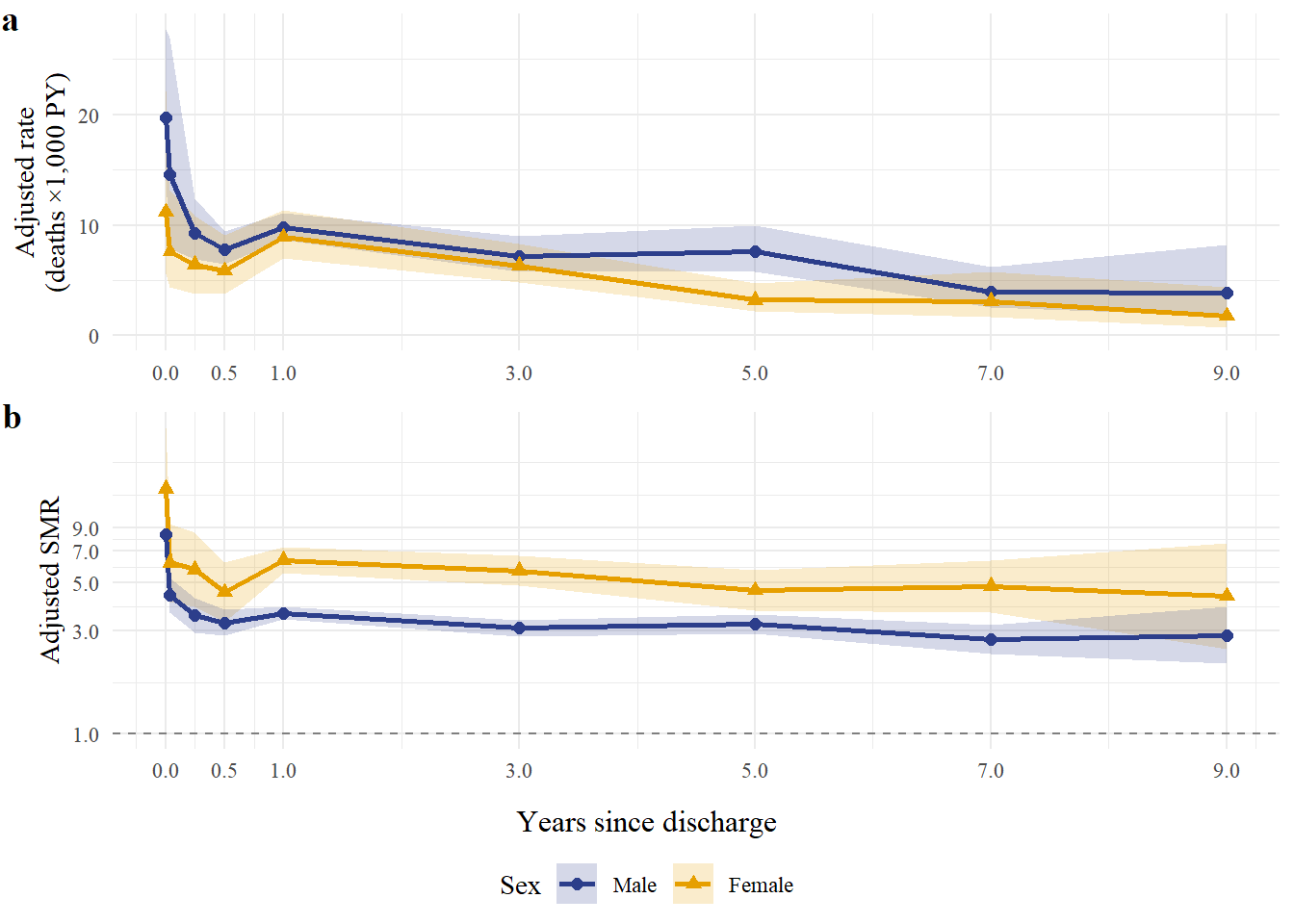
Code
figexp<- 1.5
deinflar_word <- 1/1.07653631284916
ggsave(
paste0(gsub("/cons","",getwd()), "/cons/_figs/Figure_1_rates_and_SIR_by_fot_updated_postrev.pdf"),
dpi = 600,
width = 80 *figexp,
height = 80 * figexp* (7/6),
units = "mm",
device = cairo_pdf
)
ggsave(
paste0(gsub("/cons","",getwd()), "/cons/_figs/Figure_1_rates_and_SIR_by_fot_updated_postrev.png"),
dpi = 600,
width = 80 *figexp*deinflar_word,
height = 80 * figexp*deinflar_word* (7/6),
units = "mm"
)
Summary statistics
Code
cat("Nearly inmediate deaths\n")
scales::percent((9+22+40+113)/2996, accuracy=.1)

clean_df |>
mutate(fu_years = as.numeric(difftime(death_date_rec, disch_date_rec6, units = "days")) / 365.2425) |>
summarise(
median = sprintf("%1.2f",median(fu_years)),
q25 = sprintf("%1.2f",quantile(fu_years, 0.25)),
q75 = sprintf("%1.2f",quantile(fu_years, 0.75))
)
Nearly inmediate deaths
[1] "6.1%"
median q25 q75
1 4.90 2.76 7.19Sensitivity, last treatment
Overall, age, sex
Code
## SMR, Overall  -----------------------------------------------------------
c_SISTRAT_b_std_bins <- lexpand(
  clean_df_b,
  status = status,
  birth = birth_date_rec,
  exit = death_date_rec,
  entry = disch_date_rec6,
  breaks = list(
    per = seq(2010, 2021, by = 1),
    age = age_breaks # <--- This matches the reference keys (15, 20, 25...)
  ),
  aggre = list(year = per,
               agegroup = age,
               sex = sex_rec)
)


sir_final_b_std <- popEpi::sir(
  coh.data = c_SISTRAT_b_std_bins,
  coh.obs = 'from0to1',    # Observed deaths column
  coh.pyrs = 'pyrs',       # Person-years column
  ref.data = mx_national_clean,
  ref.rate = 'mx',         # The mortality rate column in reference
  adjust = c('agegroup', 'year', 'sex')#,
#print = 'total'
)
print(sir_final_b_std)

sir_ci_phi_improved( sir_final_b_std, extract_phi(c_SISTRAT_b_std_bins)) |>
  dplyr::mutate(print= sprintf("%.2f (%.2f–%.2f)",
  SIR,
  CI_low,
  CI_high)) |>
  data.table::data.table()
SIR (adjusted by agegroup, year, sex) with 95% confidence intervals (profile)
Total sir: 4.01 (3.87-4.16)
Total observed: 3029
Total expected: 754.55
Total person-years: 317628
observed expected pyrs sir sir.lo sir.hi p_value
<num> <num> <num> <num> <num> <num> <num>
1: 3029 754.55 317627.6 4.01 3.87 4.16 0
SIR CI_low CI_high phi_used print
<num> <num> <num> <num> <char>
1: 4.014304 3.873862 4.159838 1 4.01 (3.87–4.16)Code
## DSRs  -----------------------------------------------------------
dsr_tot_b <- popEpi::rate(
data    = c_SISTRAT_b_std_bins,
obs     = "from0to1",
pyrs    = "pyrs",
adjust  = c("year","sex","agegroup"),
weights = weights_corr
)
dsr_tot_b$rate_1k <- dsr_tot_b$rate * 1e3
DSR_1k_corr_corr_b <- base::mapply(
  dsr_format_corr,                 # FUN
  dsr_tot_b$rate.adj,           # primer vector (rate)
  dsr_tot_b$SE.rate.adj,        # segundo vector (se)
  MoreArgs = list(            # argumentos fijos extra
    #phi    = extract_phi_dir(c_SISTRAT_std_bins),
    #opc. conservadora
    phi    = base::max(1,  extract_phi_dir(c_SISTRAT_b_std_bins)),
    factor = 1e3,
    digits = 1,
    conf   = 0.95))
#DSR_1k_corr_corr_b
#[1] "12.1 (9.7–15.2)"
Code
## DSR w/ 5-yr-bin lexis, unfinished tr.- by old ages -------------------------------------------
### DSR, by age ---------------------------
c_SISTRAT_b_std_old <- c_SISTRAT_b_std_bins |>
  dplyr::mutate(agegroup_old = to_old_agegroup(agegroup)) |>
  dplyr::group_by(year, sex, agegroup_old) |>
  dplyr::summarise(
  pyrs     = base::sum(pyrs),
  from0to1 = base::sum(from0to1),
  .groups  = "drop"
)
dsr_age_old_b <- popEpi::rate(
  data    = c_SISTRAT_b_std_old,
  obs     = "from0to1",
  pyrs    = "pyrs",
  print   = "agegroup_old",
  adjust  = c("year","sex"),
  weights = list(year = w_year, sex = w_sex)
)
#### Etract phi ---------------------------
phi_df_age_old_b <- extract_phi_by_age(c_SISTRAT_b_std_old|> dplyr::rename(agegroup = agegroup_old))
phi_vec_age_old_b <- base::pmax(1, phi_df_age_old_b$phi[match(dsr_age_old_b$agegroup_old, phi_df_age_old_b$agegroup)])
#### Combine phi ---------------------------
dsr_age_old_b<- cbind.data.frame(dplyr::as_tibble(dsr_age_old_b),phi= phi_vec_age_old_b)
# dplyr::select(dsr_age_old_b, rate, rate.lo, rate.hi)|>
# mutate_if(is.numeric, ~sprintf("%1.1f",.*1e3))

DSR_1k_corr_agegr_corr_b <- base::mapply(
  dsr_format_corr,
  dsr_age_old_b$rate.adj,
  dsr_age_old_b$SE.rate.adj,
  dsr_age_old_b$phi,
  MoreArgs = list(factor = 1e3, digits = 6, conf = .95)
  )
Code
### SMR by old ages ---------------------------
c_SISTRAT_b_std_bins_wold <- c_SISTRAT_b_std_bins |>
dplyr::mutate(agegroup_old = to_old_agegroup(agegroup))

smr_age_old_b <-
  popEpi::sir(c_SISTRAT_b_std_bins_wold, coh.obs = 'from0to1',
    coh.pyrs = 'pyrs',
    ref.data = mx_national_clean,
    ref.rate = mx,
    print = c("agegroup_old"),
    adjust = c("year", "sex", "agegroup"), #2025-12-16: the original still adjusts for agegroup
    test.type = "homogeneity",
    conf.type = "wald", #conf.type = "wald" usa la aproximación normal de Poisson (la misma lógica que explicamos antes).
    conf.level = 0.95, EAR = T)

# sir_ci_phi_improved( smr_age_old_b, dsr_age_old_b$phi)|>
# dplyr::mutate(print= sprintf("%.2f (%.2f–%.2f)",
# SIR,
# CI_low,
# CI_high)) |>
# data.table::data.table()
Code
## DSR w/ 5-yr-bin lexis, unfinished tr.- by sex -------------------------------------------
### DSR by sex--------------------------
phi_sex_df_b  <- extract_phi_by_sex(c_SISTRAT_b_std_bins)
dsr_by_sex_b <- popEpi::rate(
  data    = c_SISTRAT_b_std_bins,
  obs     = "from0to1",
  pyrs    = "pyrs",
  print   = "sex",
  adjust  = c("year","agegroup"),
    weights = list(year = w_year_5y, agegroup = w_age_5y)
  )
# dplyr::select(dsr_by_sex_b, rate, rate.lo, rate.hi)|>
# mutate_if(is.numeric, ~sprintf("%1.1f",.*1e3))

phi_sex_vec_b <- base::pmax(1, phi_sex_df_b$phi[match(dsr_by_sex_b$sex, phi_sex_df_b$sex)])
dsr_by_sex_b <- cbind.data.frame(dplyr::as_tibble(dsr_by_sex_b),phi= phi_sex_vec_b)
DSR_1k_corr_sex_corr_b <- base::mapply(
  dsr_format_corr,
  dsr_by_sex_b $rate.adj,
  dsr_by_sex_b $SE.rate.adj,
  phi     = 1, #not necessary (phis <1)
    MoreArgs = list(factor = 1e3, digits = 6, conf = .95)
  )

# data.table::data.table(as.vector(sapply(DSR_1k_corr_sex_corr_b,
# format_interval)))
Code
### SMR by sex--------------------------
smr_sex_corr_b <- popEpi::sir(
coh.data = c_SISTRAT_b_std_bins,
coh.obs  = "from0to1",
coh.pyrs = "pyrs",
ref.data = mx_national_clean,
ref.rate = "mx",
print    = "sex",
adjust   = c("year","sex","agegroup")  # <- 5y internal
)
smr_sex_corr_b

smr_sex_corr_tbl_b <- cbind.data.frame(dplyr::as_tibble(smr_sex_corr_b), phi=phi_sex_vec_b)
# smr_sex_corr_tbl_b

# sir_ci_phi_improved( smr_sex_corr_b, smr_sex_corr_tbl_b$phi)|>
# dplyr::mutate(print= sprintf("%.2f (%.2f–%.2f)",
# SIR,
# CI_low,
# CI_high)) |>
# data.table::data.table()
SIR (adjusted by year, sex, agegroup) with 95% confidence intervals (profile)
Test for homogeneity: p < 0.001
Total sir: 4.01 (3.87-4.16)
Total observed: 3029
Total expected: 754.55
Total person-years: 317628
Clave <sex>
sex observed expected pyrs sir sir.lo sir.hi p_value
<char> <num> <num> <num> <num> <num> <num> <num>
1: Female 604 98.77 75044.33 6.12 5.64 6.62 0
2: Male 2425 655.78 242583.25 3.70 3.55 3.85 0Code
# -------------------------
# OVERALL
# -------------------------
sir_overall_ci_b <- sir_ci_phi_improved(sir_final_b_std, extract_phi(c_SISTRAT_b_std_bins)) |>
  dplyr::mutate(SMR = fmt_interval(base::sprintf("%.2f (%.2f–%.2f)", SIR, CI_low, CI_high)))

overall_tbl_b <- data.frame(
  Section = "Overall",
  Subgroup = "All",
  `Obs/Exp` = base::paste0(sir_final_b_std$observed[1], "/", base::as.integer(sir_final_b_std$expected[1])),
  `Person-years` = base::formatC(sir_final_b_std$pyrs[1], format="f", digits=0, big.mark=","),
  phi = base::sprintf("%1.2f", base::max(1, extract_phi_dir(c_SISTRAT_b_std_bins))),
  SMR = sir_overall_ci_b$SMR[1],
  DSR_1k = fmt_interval(DSR_1k_corr_corr_b[1]),
  CMR_1k = cmr_1k_print(dsr_tot_b$rate[1], dsr_tot_b$rate.lo[1], dsr_tot_b$rate.hi[1], digits = 1),
  stringsAsFactors = FALSE
)

# -------------------------
# SEX
# -------------------------
smr_sex_corr_b <- smr_sex_corr_b[
  base::match(dsr_by_sex_b$sex, smr_sex_corr_b$sex),
]
sir_sex_ci_b <- sir_ci_phi_improved(smr_sex_corr_b, smr_sex_corr_tbl_b$phi) |>
  dplyr::mutate(SMR = fmt_interval(base::sprintf("%.2f (%.2f–%.2f)", SIR, CI_low, CI_high)))

dsr_sex_str_b <- fmt_interval(base::as.vector(base::sapply(DSR_1k_corr_sex_corr_b, format_interval)))

smr_sex_corr_tbl_b <- smr_sex_corr_tbl_b[
  base::match(dsr_by_sex_b$sex, smr_sex_corr_tbl_b$sex),
]

sex_tbl_b <- data.frame(
  Section = "Sex",
  Subgroup = base::as.character(dsr_by_sex_b$sex),
  `Obs/Exp` = base::paste0(smr_sex_corr_tbl_b$observed, "/", base::as.integer(smr_sex_corr_tbl_b$expected)),
  `Person-years` = base::formatC(dsr_by_sex_b$pyrs, format="f", digits=0, big.mark=","),
  phi = base::sprintf("%1.2f", dsr_by_sex_b$phi),
  SMR = sir_sex_ci_b$SMR,
  DSR_1k = dsr_sex_str_b,
  CMR_1k = cmr_1k_print(dsr_by_sex_b$rate, dsr_by_sex_b$rate.lo, dsr_by_sex_b$rate.hi, digits = 1),
  stringsAsFactors = FALSE
)

# -------------------------
# AGE (old bins)
# -------------------------
sir_age_ci_b <- sir_ci_phi_improved(smr_age_old_b, dsr_age_old_b$phi) |>
  dplyr::mutate(SMR = fmt_interval(base::sprintf("%.2f (%.2f–%.2f)", SIR, CI_low, CI_high)))

dsr_age_str_b <- fmt_interval(base::as.vector(base::sapply(DSR_1k_corr_agegr_corr_b, format_interval)))

age_tbl_b <- data.frame(
  Section = "Age group",
  Subgroup = base::as.character(dsr_age_old_b$agegroup_old),
  `Obs/Exp` = base::paste0(smr_age_old_b$observed, "/", base::as.integer(smr_age_old_b$expected)),
  `Person-years` = base::formatC(dsr_age_old_b$pyrs, format="f", digits=0, big.mark=","),
  phi = base::sprintf("%1.2f", dsr_age_old_b$phi),
  SMR = sir_age_ci_b$SMR,
  DSR_1k = dsr_age_str_b,
  CMR_1k = cmr_1k_print(dsr_age_old_b$rate, dsr_age_old_b$rate.lo, dsr_age_old_b$rate.hi, digits = 1),
  stringsAsFactors = FALSE
)

# -------------------------
# FINAL
# -------------------------
final_tbl_b <- base::rbind(overall_tbl_b, sex_tbl_b, age_tbl_b)

knitr::kable(
  final_tbl_b,
  caption = "Sensitivity 1: Summary of SMR (phi-corrected), DSR and CMR (per 1,000 person-years) overall and by sex/age.",
  align = c("l","l","l","r","r","l","l","l")
)| Section | Subgroup | Obs.Exp | Person.years | phi | SMR | DSR_1k | CMR_1k |
|---|---|---|---|---|---|---|---|
| Overall | All | 3029/754 | 317,628 | 1.00 | 4.01 (3.87–4.16) | 12.1 (9.7–15.2) | 9.5 (9.2–9.9) |
| Sex | Male | 2425/655 | 242,583 | 1.00 | 3.70 (3.55–3.85) | 15.7 (10.6–23.3) | 10.0 (9.6–10.4) |
| Sex | Female | 604/98 | 75,044 | 1.00 | 6.11 (5.65–6.62) | 9.0 (7.4–11.0) | 8.0 (7.4–8.7) |
| Age group | 18 | 222/60 | 66,757 | 1.00 | 3.64 (3.19–4.16) | 3.6 (3.0–4.5) | 3.3 (2.9–3.8) |
| Age group | 30 | 1097/244 | 163,996 | 1.22 | 4.50 (4.21–4.80) | 7.3 (5.7–9.3) | 6.7 (6.3–7.1) |
| Age group | 45 | 1351/316 | 75,900 | 1.00 | 4.27 (4.05–4.51) | 16.3 (14.7–18.2) | 17.8 (16.9–18.8) |
| Age group | 60 | 359/133 | 10,975 | 1.00 | 2.69 (2.43–2.98) | 53.5 (21.5–133.2) | 32.7 (29.5–36.3) |
Heterogeneity
Code
smr_sex_dat_b <- sir_ci_phi_improved( smr_sex_corr_b, smr_sex_corr_tbl_b$phi) |>
    dplyr::mutate(
        yi  = base::log(SIR),
        sei = se_log_from_ci(SIR, CI_low, CI_high, conf = 0.95)
    )

meta_smr_sex_b <- metafor::rma(
    yi = yi,
    sei = sei,
    method = "FE",
    data = smr_sex_dat_b
)

smr_age_dat_b <- sir_ci_phi_improved( smr_age_old_b, sir_age_ci_b$phi) |>
    dplyr::mutate(
        yi  = base::log(SIR),
        sei = se_log_from_ci(SIR,CI_low, CI_high, conf = 0.95)
    )

meta_smr_age_b <- metafor::rma(
    yi = yi,
    sei = sei,
    method = "FE",
    data = smr_age_dat_b
)

dsr_sex_dat_b <- dsr_by_sex_b |>
    dplyr::mutate(sex = base::as.character(sex)) |>
    dplyr::mutate(
        yi  = base::log(rate.adj),
        sei = se_log_from_rate_se(rate.adj, SE.rate.adj, phi = phi)
    )

meta_dsr_sex_b <- metafor::rma(
    yi = yi,
    sei = sei,
    method = "FE",
    data = dsr_sex_dat_b
)

dsr_age_dat_b <- dsr_age_old_b |>
    dplyr::mutate(
        yi  = base::log(rate.adj),
        sei = se_log_from_rate_se(rate.adj, SE.rate.adj, phi = phi)
    )

meta_dsr_age_b <- metafor::rma(yi = yi, sei = sei, method = "FE", data = dsr_age_dat_b)


het_tbl_b <- base::rbind(
  het_row(meta_smr_sex_b, "SMR (SIR) by sex"),
  het_row(meta_smr_age_b, "SMR (SIR) by age group"),
  het_row(meta_dsr_sex_b, "DSR by sex"),
  het_row(meta_dsr_age_b, "DSR by age group")
)

knitr::kable(
  het_tbl_b,
  caption = "Heterogeneity tests (fixed-effect meta-analysis; Cochran’s Q and I²).",
  align = c("l","r","r","r","r")
)| Analysis | Q | df | p | I2 |
|---|---|---|---|---|
| SMR (SIR) by sex | 122.33 | 1 | 0.000 | 99.2 |
| SMR (SIR) by age group | 76.09 | 3 | 0.000 | 96.1 |
| DSR by sex | 6.18 | 1 | 0.013 | 83.8 |
| DSR by age group | 188.17 | 3 | 0.000 | 98.4 |
Reformat Lexis
Code
## By strata, last tr. -----------------------------------------------------
clean_df2_b <- clean_df_b |>
  dplyr::mutate(
  # 0/1 -> labels ( 1 = Residential, 0 = Ambulatory)
  setting = dplyr::if_else(res_plan == 1, "Residential", "Ambulatory"),
  setting = base::factor(setting, levels = c("Ambulatory","Residential")),
  completed = base::as.character(tr_compliance_status),
  completed = base::factor(completed, levels = c("Completed","Not completed")),
  licit_illicit = base::as.character(prim_sub_licit),
  licit_illicit = base::factor(licit_illicit, levels = c("licit","illicit")),
  disch_age_cat = base::as.character(disch_age_cat),
  disch_age_cat = base::factor(disch_age_cat, levels = c("18-29","30-44","45-59","60+")),
  # Sex: asegúrate que sea Male/Female como tus tasas nacionales
  sex = stringr::str_to_title(base::as.character(sex_rec)),
  sex = base::factor(sex, levels = c("Male","Female"))
)
# ---- 2) 5-year attained-age Lexis (keep 2021 as boundary)
c_SISTRAT_5y_b <- popEpi::lexpand(
  data   = clean_df2_b,
  status = status,
  birth  = birth_date_rec,
  entry  = disch_date_rec6,
  exit   = death_date_rec,
  breaks = list(
  per = base::seq(2010, 2021, by = 1),
  age = age_breaks
  ),
  aggre = list(
  year    = per,
  agegroup= age,      # 5y attained-age keys (15,20,25,...)
  sex     = sex,
  # subgroup vars (constantes por individuo; quedan replicadas por split)
  setting      = setting,
  completed    = completed,
  licit_illicit= licit_illicit,
  disch_age_cat= disch_age_cat
  )
)
Strata
DSR
Code
dsr_setting_b   <- run_dsr_by(c_SISTRAT_5y_b, weights_corr, "setting")
dsr_completed_b <- run_dsr_by(c_SISTRAT_5y_b, weights_corr, "completed")
dsr_licit_b     <- run_dsr_by(c_SISTRAT_5y_b, weights_corr, "licit_illicit")
Code
tbl_all_b <- base::rbind(
    prep_dsr(dsr_setting_b,   "Setting"),
    prep_dsr(dsr_completed_b, "Completion"),
    prep_dsr(dsr_licit_b,     "Licit/illicit")#,  prep_dsr(dsr_age,       "Age group")
)

knitr::kable(
    tbl_all_b,
    caption = "Directly standardized rates (DSR) and crude mortality rates (CMR), per 1,000 person-years, across subgroups.",
    align = c("l","l","r","r","r","r","r","l","r","r","r","r")
)| Section | Group | Deaths | Person-years | DSR/1,000 | DSR L | DSR U | DSR/1,000 (95% CI) | CMR/1,000 | CMR L | CMR U | Phi |
|---|---|---|---|---|---|---|---|---|---|---|---|
| Setting | Ambulatory | 2452 | 268,495.4 | 11.65 | 8.90 | 15.24 | 11.65 (8.90–15.24) | 9.13 | 8.78 | 9.50 | 1.341 |
| Setting | Residential | 577 | 49,132.2 | 12.85 | 9.88 | 16.71 | 12.85 (9.88–16.71) | 11.74 | 10.82 | 12.74 | 1.336 |
| Completion | Completed | 716 | 81,225.8 | 8.64 | 6.53 | 11.44 | 8.64 (6.53–11.44) | 8.81 | 8.19 | 9.48 | 1.584 |
| Completion | Not completed | 2313 | 236,401.7 | 13.63 | 10.12 | 18.36 | 13.63 (10.12–18.36) | 9.78 | 9.39 | 10.19 | 1.641 |
| Licit/illicit | licit | 1787 | 98,631.2 | 14.94 | 12.34 | 18.08 | 14.94 (12.34–18.08) | 18.12 | 17.30 | 18.98 | 1.628 |
| Licit/illicit | illicit | 1242 | 218,996.3 | 10.56 | 6.31 | 17.66 | 10.56 (6.31–17.66) | 5.67 | 5.36 | 6.00 | 1.000 |
SMR
Code
smr_setting_b   <- run_smr_by(c_SISTRAT_5y_b, mx_national_clean, "setting")
smr_completed_b <- run_smr_by(c_SISTRAT_5y_b, mx_national_clean, "completed")
smr_licit_b     <- run_smr_by(c_SISTRAT_5y_b, mx_national_clean, "licit_illicit")


smr_setting_phi_b <- smr_setting_b%>%
    dplyr::left_join(dplyr::select(dsr_setting_b, group, phi), by = "group")%>%
    sir_ci_phi_profile(phi = .$phi) |>
    dplyr::mutate(print = sprintf(paste0("%.", 2, "f (%.", 2, "f–%.", 2, "f)"),
                                  sir, sir.phi.lo, sir.phi.hi))
smr_completed_phi_b <- smr_completed_b%>%
    dplyr::left_join(dplyr::select(dsr_completed_b, group, phi), by = "group")%>%
    sir_ci_phi_profile(phi = .$phi) |>
    dplyr::mutate(print = sprintf(paste0("%.", 2, "f (%.", 2, "f–%.", 2, "f)"),
                                  sir, sir.phi.lo, sir.phi.hi))
smr_licit_phi_b <- smr_licit_b%>%
    dplyr::left_join(dplyr::select(dsr_licit_b, group, phi), by = "group")%>%
    sir_ci_phi_profile(phi = .$phi) |>
    dplyr::mutate(print = sprintf(paste0("%.", 2, "f (%.", 2, "f–%.", 2, "f)"),
                                  sir, sir.phi.lo, sir.phi.hi))
# Combine all tables into one with a "Category" column
smr_table_b <- bind_rows(
    smr_setting_phi_b %>% mutate(Category = "Setting") %>% dplyr::select(Category, Group = group, Observed = observed, Expected = expected, SMR = print),
    smr_completed_phi_b %>% mutate(Category = "Treatment Completion") %>% dplyr::select(Category, Group = group, Observed = observed, Expected = expected, SMR = print),
    smr_licit_phi_b %>% mutate(Category = "Primary Substance") %>% dplyr::select(Category, Group = group, Observed = observed, Expected = expected, SMR = print)#,
    # smr_agecat_phi %>% mutate(Category = "Age at Discharge") %>% select(Category, Group = group, Observed = observed, Expected = expected, SMR = print)
) %>%
    dplyr::mutate(Category = ifelse( Category != lag(Category, default = ""),
            Category,
            ""))

# Create kable
kable(
    smr_table_b,
    col.names = c("Category", "Group", "Observed", "Expected", "SMR (95% CI)"),
    align = c("l", "l", "r", "r", "r"),
    booktabs = TRUE,
    linesep = ""
) | Category | Group | Observed | Expected | SMR (95% CI) |
|---|---|---|---|---|
| Setting | Ambulatory | 2452 | 652.9790 | 3.76 (3.59–3.93) |
| Residential | 577 | 101.5727 | 5.68 (5.17–6.24) | |
| Treatment Completion | Completed | 716 | 241.8276 | 2.96 (2.70–3.25) |
| Not completed | 2313 | 512.7241 | 4.51 (4.28–4.75) | |
| Primary Substance | licit | 1787 | 353.2577 | 5.06 (4.77–5.37) |
| illicit | 1242 | 401.2941 | 3.10 (2.93–3.27) |
Heterogeneity
Code
# --- 1) Run SMRs ----------------------------------------------------------
smr_setting_b   <- run_smr_by(c_SISTRAT_5y_b, mx_national_clean, "setting")
smr_completed_b <- run_smr_by(c_SISTRAT_5y_b, mx_national_clean, "completed")
smr_licit_b     <- run_smr_by(c_SISTRAT_5y_b, mx_national_clean, "licit_illicit")

# --- 2) Phi-corrected SMRs (profile CI) ----------------------------------
smr_setting_phi_b   <- make_smr_phi(smr_setting_b,   dsr_setting_b)
smr_completed_phi_b <- make_smr_phi(smr_completed_b, dsr_completed_b)
smr_licit_phi_b     <- make_smr_phi(smr_licit_b,     dsr_licit_b)

# --- 3) Heterogeneity helper (DSR + SMR) ---------------------------------


# --- 4) Fit meta models ---------------------------------------------------
meta_dsr_setting_b <- het_dsr(dsr_setting_b)
meta_smr_setting_b <- het_smr(smr_setting_phi_b)

meta_dsr_compl_b   <- het_dsr(dsr_completed_b)
meta_smr_compl_b   <- het_smr(smr_completed_phi_b)

meta_dsr_licit_b   <- het_dsr(dsr_licit_b)
meta_smr_licit_b   <- het_smr(smr_licit_phi_b)

# --- 5) Print quick heterogeneity table ----------------------------------
het_tbl_b <- base::rbind(
  het_row_strata(meta_dsr_setting_b, "Setting",       "DSR"),
  het_row_strata(meta_smr_setting_b, "Setting",       "SMR"),
  het_row_strata(meta_dsr_compl_b,   "Compliance",    "DSR"),
  het_row_strata(meta_smr_compl_b,   "Compliance",    "SMR"),
  het_row_strata(meta_dsr_licit_b,   "Licit/Illicit", "DSR"),
  het_row_strata(meta_smr_licit_b,   "Licit/Illicit", "SMR")
)

knitr::kable(
  het_tbl_b,
  caption = "Heterogeneity tests (fixed-effect meta-analysis): Cochran’s Q and I² (phi-corrected).",
  align = c("l","l","r","r","r","r")
)| Contrast | Outcome | Q | df | p | I2 |
|---|---|---|---|---|---|
| Setting | DSR | 0.26 | 1 | 0.608 | 0.0 |
| Setting | SMR | 59.87 | 1 | 0.000 | 98.3 |
| Compliance | DSR | 4.76 | 1 | 0.029 | 79.0 |
| Compliance | SMR | 60.69 | 1 | 0.000 | 98.4 |
| Licit/Illicit | DSR | 1.54 | 1 | 0.215 | 34.9 |
| Licit/Illicit | SMR | 140.64 | 1 | 0.000 | 99.3 |
Sensitivity, unfinished treatments
Overall, age, sex
Code
## SMR, Overall  -----------------------------------------------------------
c_SISTRAT_c_std_bins <- popEpi::lexpand(
  clean_df_c,
  status = status,
  birth = birth_date_rec,
  exit = death_date_rec,
  entry = disch_date_corr,
  breaks = list(
  per = seq(2010, 2021, by = 1),
  age = age_breaks # <--- This matches the reference keys (15, 20, 25...)
  ),
    aggre = list(year = per,
    agegroup = age,
    sex = sex_rec)
)

sir_final_c_std <- popEpi::sir(
  coh.data = c_SISTRAT_c_std_bins,
  coh.obs = 'from0to1',    # Observed deaths column
  coh.pyrs = 'pyrs',       # Person-years column
  ref.data = mx_national_clean,
  ref.rate = 'mx',         # The mortality rate column in reference
  adjust = c('agegroup', 'year', 'sex')#,
#print = 'total'
)
print(sir_final_c_std)

sir_ci_phi_improved( sir_final_c_std, extract_phi(c_SISTRAT_c_std_bins)) |>
  dplyr::mutate(print= sprintf("%.2f (%.2f–%.2f)",
  SIR,
  CI_low,
  CI_high)) |>
  data.table::data.table()
SIR (adjusted by agegroup, year, sex) with 95% confidence intervals (profile)
Total sir: 4 (3.88-4.13)
Total observed: 3817
Total expected: 953.61
Total person-years: 416286
observed expected pyrs sir sir.lo sir.hi p_value
<num> <num> <num> <num> <num> <num> <num>
1: 3817 953.61 416285.6 4 3.88 4.13 0
SIR CI_low CI_high phi_used print
<num> <num> <num> <num> <char>
1: 4.002704 3.877715 4.131721 1 4.00 (3.88–4.13)Code
## DSRs  -----------------------------------------------------------
dsr_tot_c <- popEpi::rate(
data    = c_SISTRAT_c_std_bins,
obs     = "from0to1",
pyrs    = "pyrs",
adjust  = c("year","sex","agegroup"),
weights = weights_corr
)
dsr_tot_c$rate_1k <- dsr_tot_c$rate * 1e3
DSR_1k_corr_corr_c <- base::mapply(
  dsr_format_corr,                 # FUN
  dsr_tot_c$rate.adj,           # primer vector (rate)
  dsr_tot_c$SE.rate.adj,        # segundo vector (se)
  MoreArgs = list(            # argumentos fijos extra
    #phi    = extract_phi_dir(c_SISTRAT_std_bins),
    #opc. conservadora
    phi    = base::max(1,  extract_phi_dir(c_SISTRAT_c_std_bins)),
    factor = 1e3,
    digits = 1,
    conf   = 0.95))
# DSR_1k_corr_corr_c
# [1] "11.2 (10.0–12.5)"
Code
## DSR w/ 5-yr-bin lexis, unfinished tr.- by old ages -------------------------------------------
### DSR, by age ---------------------------
c_SISTRAT_c_std_old <- c_SISTRAT_c_std_bins |>
dplyr::mutate(agegroup_old = to_old_agegroup(agegroup)) |>
dplyr::group_by(year, sex, agegroup_old) |>
dplyr::summarise(
pyrs     = base::sum(pyrs),
from0to1 = base::sum(from0to1),
.groups  = "drop"
)
dsr_age_old_c <- popEpi::rate(
data    = c_SISTRAT_c_std_old,
obs     = "from0to1",
pyrs    = "pyrs",
print   = "agegroup_old",
adjust  = c("year","sex"),
weights = list(year = w_year, sex = w_sex)
)
#### Etract phi ---------------------------
phi_df_age_old_c <- extract_phi_by_age(c_SISTRAT_c_std_old|> dplyr::rename(agegroup = agegroup_old))
phi_vec_age_old_c <- base::pmax(1, phi_df_age_old_c$phi[match(dsr_age_old_c$agegroup_old, phi_df_age_old_c$agegroup)])
#### Combine phi ---------------------------
dsr_age_old_c<- cbind.data.frame(dplyr::as_tibble(dsr_age_old_c),phi= phi_vec_age_old_c)
# dplyr::select(dsr_age_old_c, rate, rate.lo, rate.hi)|>
# mutate_if(is.numeric, ~sprintf("%1.1f",.*1e3))

DSR_1k_corr_agegr_corr_c <- base::mapply(
  dsr_format_corr,
  dsr_age_old_c$rate.adj,
  dsr_age_old_c$SE.rate.adj,
  dsr_age_old_c$phi,
  MoreArgs = list(factor = 1e3, digits = 6, conf = .95)
  )

# data.table::data.table(as.vector(sapply(DSR_1k_corr_agegr_corr_c,
# format_interval)))
Code
### SMR by old ages ---------------------------
c_SISTRAT_c_std_bins_wold <- c_SISTRAT_c_std_bins |>
dplyr::mutate(agegroup_old = to_old_agegroup(agegroup))

smr_age_old_c <-
  popEpi::sir(c_SISTRAT_c_std_bins_wold, coh.obs = 'from0to1',
    coh.pyrs = 'pyrs',
    ref.data = mx_national_clean,
    ref.rate = mx,
    print = c("agegroup_old"),
    adjust = c("year", "sex", "agegroup"), #2025-12-16: the original still adjusts for agegroup
    test.type = "homogeneity",
    conf.type = "wald", #conf.type = "wald" usa la aproximación normal de Poisson (la misma lógica que explicamos antes).
    conf.level = 0.95, EAR = T)
# sir_ci_phi_improved( smr_age_old_c, dsr_age_old_c$phi)|>
#   dplyr::mutate(print= sprintf("%.2f (%.2f–%.2f)",
#   SIR,
#   CI_low,
#   CI_high)) |>
#   data.table::data.table()
Code
## DSR w/ 5-yr-bin lexis, unfinished tr.- by sex -------------------------------------------
### DSR by sex--------------------------
phi_sex_df_c  <- extract_phi_by_sex(c_SISTRAT_c_std_bins)
dsr_by_sex_c <- popEpi::rate(
  data    = c_SISTRAT_c_std_bins,
  obs     = "from0to1",
  pyrs    = "pyrs",
  print   = "sex",
  adjust  = c("year","agegroup"),
  weights = list(year = w_year_5y, agegroup = w_age_5y)
  )
# dplyr::select(dsr_by_sex_c, rate, rate.lo, rate.hi)|>
# mutate_if(is.numeric, ~sprintf("%1.1f",.*1e3))

phi_sex_vec_c <- base::pmax(1, phi_sex_df_c$phi[match(dsr_by_sex_c$sex, phi_sex_df_c$sex)])
dsr_by_sex_c <- cbind.data.frame(dplyr::as_tibble(dsr_by_sex_c),phi= phi_sex_vec_c)
DSR_1k_corr_sex_corr_c <- base::mapply(
dsr_format_corr,
dsr_by_sex_c $rate.adj,
dsr_by_sex_c $SE.rate.adj,
phi     = 1, #not necessary (phis <1)
MoreArgs = list(factor = 1e3, digits = 6, conf = .95)
)
#
# data.table::data.table(as.vector(sapply(DSR_1k_corr_sex_corr_c,
# format_interval)))
Code
### SMR by sex--------------------------
smr_sex_corr_c <- popEpi::sir(
coh.data = c_SISTRAT_c_std_bins,
coh.obs  = "from0to1",
coh.pyrs = "pyrs",
ref.data = mx_national_clean,
ref.rate = "mx",
print    = "sex",
adjust   = c("year","sex","agegroup")  # <- 5y internal
)
smr_sex_corr_c

smr_sex_corr_tbl_c <- cbind.data.frame(dplyr::as_tibble(smr_sex_corr_c), phi=phi_sex_vec_c)
# smr_sex_corr_tbl_c
#
# sir_ci_phi_improved( smr_sex_corr_c, smr_sex_corr_tbl_c$phi)|>
#   dplyr::mutate(print= sprintf("%.2f (%.2f–%.2f)",
#   SIR,
#   CI_low,
#   CI_high)) |>
#   data.table::data.table()
SIR (adjusted by year, sex, agegroup) with 95% confidence intervals (profile)
Test for homogeneity: p < 0.001
Total sir: 4 (3.88-4.13)
Total observed: 3817
Total expected: 953.61
Total person-years: 416286
Clave <sex>
sex observed expected pyrs sir sir.lo sir.hi p_value
<char> <num> <num> <num> <num> <num> <num> <num>
1: Female 805 134.91 106197.2 5.97 5.56 6.39 0
2: Male 3012 818.70 310088.4 3.68 3.55 3.81 0Code
# -------------------------
# OVERALL
# -------------------------
sir_overall_ci_c <- sir_ci_phi_improved(sir_final_c_std, extract_phi(c_SISTRAT_c_std_bins)) |>
  dplyr::mutate(SMR = fmt_interval(base::sprintf("%.2f (%.2f–%.2f)", SIR, CI_low, CI_high)))

overall_tbl_c <- data.frame(
  Section = "Overall",
  Subgroup = "All",
  `Obs/Exp` = base::paste0(sir_final_c_std$observed[1], "/", base::as.integer(sir_final_c_std$expected[1])),
  `Person-years` = base::formatC(sir_final_c_std$pyrs[1], format="f", digits=0, big.mark=","),
  phi = base::sprintf("%1.2f", base::max(1, extract_phi_dir(c_SISTRAT_c_std_bins))),
  SMR = sir_overall_ci_c$SMR[1],
  DSR_1k = fmt_interval(DSR_1k_corr_corr_c[1]),
  CMR_1k = cmr_1k_print(dsr_tot_c$rate[1], dsr_tot_c$rate.lo[1], dsr_tot_c$rate.hi[1], digits = 1),
  stringsAsFactors = FALSE
)

# -------------------------
# SEX
# -------------------------
smr_sex_corr_c <- smr_sex_corr_c[
  base::match(dsr_by_sex_c$sex, smr_sex_corr_c$sex),
]
sir_sex_ci_c <- sir_ci_phi_improved(smr_sex_corr_c, smr_sex_corr_tbl_c$phi) |>
  dplyr::mutate(SMR = fmt_interval(base::sprintf("%.2f (%.2f–%.2f)", SIR, CI_low, CI_high)))

dsr_sex_str_c <- fmt_interval(base::as.vector(base::sapply(DSR_1k_corr_sex_corr_c, format_interval)))

smr_sex_corr_tbl_c <- smr_sex_corr_tbl_c[
  base::match(dsr_by_sex_c$sex, smr_sex_corr_tbl_c$sex),
]

sex_tbl_c <- data.frame(
  Section = "Sex",
  Subgroup = base::as.character(dsr_by_sex_c$sex),
  `Obs/Exp` = base::paste0(smr_sex_corr_tbl_c$observed, "/", base::as.integer(smr_sex_corr_tbl_c$expected)),
  `Person-years` = base::formatC(dsr_by_sex_c$pyrs, format="f", digits=0, big.mark=","),
  phi = base::sprintf("%1.2f", dsr_by_sex_c$phi),
  SMR = sir_sex_ci_c$SMR,
  DSR_1k = dsr_sex_str_c,
  CMR_1k = cmr_1k_print(dsr_by_sex_c$rate, dsr_by_sex_c$rate.lo, dsr_by_sex_c$rate.hi, digits = 1),
  stringsAsFactors = FALSE
)

# -------------------------
# AGE (old bins)
# -------------------------
sir_age_ci_c <- sir_ci_phi_improved(smr_age_old_c, dsr_age_old_c$phi) |>
  dplyr::mutate(SMR = fmt_interval(base::sprintf("%.2f (%.2f–%.2f)", SIR, CI_low, CI_high)))

dsr_age_str_c <- fmt_interval(base::as.vector(base::sapply(DSR_1k_corr_agegr_corr_c, format_interval)))

age_tbl_c <- data.frame(
  Section = "Age group",
  Subgroup = base::as.character(dsr_age_old_c$agegroup_old),
  `Obs/Exp` = base::paste0(smr_age_old_c$observed, "/", base::as.integer(smr_age_old_c$expected)),
  `Person-years` = base::formatC(dsr_age_old_c$pyrs, format="f", digits=0, big.mark=","),
  phi = base::sprintf("%1.2f", dsr_age_old_c$phi),
  SMR = sir_age_ci_c$SMR,
  DSR_1k = dsr_age_str_c,
  CMR_1k = cmr_1k_print(dsr_age_old_c$rate, dsr_age_old_c$rate.lo, dsr_age_old_c$rate.hi, digits = 1),
  stringsAsFactors = FALSE
)

# -------------------------
# FINAL
# -------------------------
final_tbl_c <- base::rbind(overall_tbl_c, sex_tbl_c, age_tbl_c)

knitr::kable(
  final_tbl_c,
  caption = "Sensitivity 2: Summary of SMR (phi-corrected), DSR and CMR (per 1,000 person-years) overall and by sex/age.",
  align = c("l","l","l","r","r","l","l","l")
)| Section | Subgroup | Obs.Exp | Person.years | phi | SMR | DSR_1k | CMR_1k |
|---|---|---|---|---|---|---|---|
| Overall | All | 3817/953 | 416,286 | 1.00 | 4.00 (3.88–4.13) | 11.2 (10.0–12.5) | 9.2 (8.9–9.5) |
| Sex | Male | 3012/818 | 310,088 | 1.00 | 3.68 (3.55–3.81) | 14.2 (11.9–16.8) | 9.7 (9.4–10.1) |
| Sex | Female | 805/134 | 106,197 | 1.00 | 5.97 (5.57–6.39) | 8.4 (7.3–9.8) | 7.6 (7.1–8.1) |
| Age group | 18 | 283/82 | 91,929 | 1.00 | 3.44 (3.06–3.86) | 2.9 (2.5–3.4) | 3.1 (2.7–3.5) |
| Age group | 30 | 1360/315 | 215,034 | 1.00 | 4.32 (4.09–4.55) | 6.2 (5.4–7.1) | 6.3 (6.0–6.7) |
| Age group | 45 | 1710/395 | 96,010 | 1.00 | 4.33 (4.13–4.54) | 16.4 (14.9–18.1) | 17.8 (17.0–18.7) |
| Age group | 60 | 464/160 | 13,312 | 1.00 | 2.88 (2.63–3.16) | 37.6 (24.6–57.4) | 34.9 (31.8–38.2) |
Heterogeneity
Code
smr_sex_dat_c <- sir_ci_phi_improved( smr_sex_corr_c, smr_sex_corr_tbl_c$phi) |>
    dplyr::mutate(
        yi  = base::log(SIR),
        sei = se_log_from_ci(SIR, CI_low, CI_high, conf = 0.95)
    )

meta_smr_sex_c <- metafor::rma(
    yi = yi,
    sei = sei,
    method = "FE",
    data = smr_sex_dat_c
)

smr_age_dat_c <- sir_ci_phi_improved( smr_age_old_c, sir_age_ci_c$phi) |>
    dplyr::mutate(
        yi  = base::log(SIR),
        sei = se_log_from_ci(SIR,CI_low, CI_high, conf = 0.95)
    )

meta_smr_age_c <- metafor::rma(
    yi = yi,
    sei = sei,
    method = "FE",
    data = smr_age_dat_c
)

dsr_sex_dat_c <- dsr_by_sex_c |>
    dplyr::mutate(sex = base::as.character(sex)) |>
    dplyr::mutate(
        yi  = base::log(rate.adj),
        sei = se_log_from_rate_se(rate.adj, SE.rate.adj, phi = phi)
    )

meta_dsr_sex_c <- metafor::rma(
    yi = yi,
    sei = sei,
    method = "FE",
    data = dsr_sex_dat_c
)

dsr_age_dat_c <- dsr_age_old_c |>
    dplyr::mutate(
        yi  = base::log(rate.adj),
        sei = se_log_from_rate_se(rate.adj, SE.rate.adj, phi = phi)
    )

meta_dsr_age_c <- metafor::rma(yi = yi, sei = sei, method = "FE", data = dsr_age_dat_c)


het_tbl_c <- base::rbind(
  het_row(meta_smr_sex_c, "SMR (SIR) by sex"),
  het_row(meta_smr_age_c, "SMR (SIR) by age group"),
  het_row(meta_dsr_sex_c, "DSR by sex"),
  het_row(meta_dsr_age_c, "DSR by age group")
)

knitr::kable(
  het_tbl_c,
  caption = "Heterogeneity tests (fixed-effect meta-analysis; Cochran’s Q and I²).",
  align = c("l","r","r","r","r")
)| Analysis | Q | df | p | I2 |
|---|---|---|---|---|
| SMR (SIR) by sex | 148.56 | 1 | 0.000 | 99.3 |
| SMR (SIR) by age group | 74.19 | 3 | 0.000 | 96.0 |
| DSR by sex | 20.11 | 1 | 0.000 | 95.0 |
| DSR by age group | 414.48 | 3 | 0.000 | 99.3 |
Reformat Lexis
Code
## By strata, unfinished tr. -----------------------------------------------------
clean_df2_c <- clean_df_c |>
dplyr::mutate(
# 0/1 -> labels ( 1 = Residential, 0 = Ambulatory)
setting = dplyr::if_else(res_plan == 1, "Residential", "Ambulatory"),
setting = base::factor(setting, levels = c("Ambulatory","Residential")),
completed = base::as.character(tr_compliance_status),
completed = base::factor(completed, levels = c("Completed","Not completed")),
licit_illicit = base::as.character(prim_sub_licit),
licit_illicit = base::factor(licit_illicit, levels = c("licit","illicit")),
disch_age_cat = base::as.character(disch_age_cat),
disch_age_cat = base::factor(disch_age_cat, levels = c("18-29","30-44","45-59","60+")),
# Sex: asegúrate que sea Male/Female como tus tasas nacionales
sex = stringr::str_to_title(base::as.character(sex_rec)),
sex = base::factor(sex, levels = c("Male","Female"))
)
# ---- 2) 5-year attained-age Lexis (keep 2021 as boundary)
table(clean_df2_c$tr_compliance_status, exclude=NULL)
# Completed Not completed          <NA>
#     19213         51047         13522
c_SISTRAT_5y_c <- popEpi::lexpand(
data   = clean_df2_c|>
dplyr::mutate(tr_compliance_status=
ifelse(is.na(tr_compliance_status),"Unfinished", tr_compliance_status)),
status = status,
birth  = birth_date_rec,
entry  = disch_date_corr,
exit   = death_date_rec,
breaks = list(
per = base::seq(2010, 2021, by = 1),
age = age_breaks
),
aggre = list(
year    = per,
agegroup= age,      # 5y attained-age keys (15,20,25,...)
sex     = sex,
# subgroup vars (constantes por individuo; quedan replicadas por split)
setting      = res_plan,
completed    = tr_compliance_status,
licit_illicit= licit_illicit,
disch_age_cat= disch_age_cat
)
)

warning("2025-12-30= I chose to separate into Unfinished and Tr. completed
")
Warning: 2025-12-30= I chose to separate into Unfinished and Tr. completedCode
c_SISTRAT_5y_c <- c_SISTRAT_5y_c |>
dplyr::mutate(
setting = factor(setting, levels = c(0, 1),
labels = c("Ambulatory", "Residential"))
)
    Completed Not completed          <NA>
        19213         51047         13522
Strata
DSR
Code
warning("disch_age_cat es edad al alta (baseline) → perfecto para “preservar
los grupos antiguos” aunque el Lexis use attained-age 5y internamente para el ajuste.")
Warning: disch_age_cat es edad al alta (baseline) → perfecto para “preservar
los grupos antiguos” aunque el Lexis use attained-age 5y internamente para el ajuste.Code
dsr_setting_c   <- run_dsr_by(c_SISTRAT_5y_c, weights_corr, "setting")
dsr_completed_c <- run_dsr_by(c_SISTRAT_5y_c, weights_corr, "completed")
Warning: There was 1 warning in `dplyr::summarise()`.
ℹ In argument: `result = list(...)`.
ℹ In group 3: `completed = "Unfinished"`.
Caused by warning:
! glm.fit: fitted rates numerically 0 occurredCode
dsr_licit_c <- run_dsr_by(c_SISTRAT_5y_c, weights_corr, "licit_illicit")Code
tbl_all_c <- base::rbind(
    prep_dsr(dsr_setting_c,   "Setting"),
    prep_dsr(dsr_completed_c, "Completion"),
    prep_dsr(dsr_licit_c,     "Licit/illicit")#,  prep_dsr(dsr_age,       "Age group")
)

knitr::kable(
    tbl_all_c,
    caption = "Directly standardized rates (DSR) and crude mortality rates (CMR), per 1,000 person-years, across subgroups.",
    align = c("l","l","r","r","r","r","r","l","r","r","r","r")
)| Section | Group | Deaths | Person-years | DSR/1,000 | DSR L | DSR U | DSR/1,000 (95% CI) | CMR/1,000 | CMR L | CMR U | Phi |
|---|---|---|---|---|---|---|---|---|---|---|---|
| Setting | Ambulatory | 3163 | 355,444.6 | 11.59 | 9.55 | 14.08 | 11.59 (9.55–14.08) | 8.90 | 8.59 | 9.21 | 1.398 |
| Setting | Residential | 654 | 60,840.9 | 10.97 | 9.19 | 13.10 | 10.97 (9.19–13.10) | 10.75 | 9.96 | 11.61 | 1.418 |
| Completion | Completed | 678 | 83,249.5 | 7.98 | 6.15 | 10.36 | 7.98 (6.15–10.36) | 8.14 | 7.55 | 8.78 | 1.628 |
| Completion | Not completed | 2476 | 270,653.7 | 12.95 | 10.12 | 16.58 | 12.95 (10.12–16.58) | 9.15 | 8.79 | 9.52 | 1.514 |
| Completion | Unfinished | 663 | 62,382.4 | 12.95 | 10.67 | 15.72 | 12.95 (10.67–15.72) | 10.63 | 9.85 | 11.47 | 1.371 |
| Licit/illicit | licit | 2240 | 124,652.9 | 14.78 | 12.90 | 16.92 | 14.78 (12.90–16.92) | 17.97 | 17.24 | 18.73 | 1.469 |
| Licit/illicit | illicit | 1577 | 291,632.7 | 9.53 | 6.61 | 13.75 | 9.53 (6.61–13.75) | 5.41 | 5.15 | 5.68 | 1.069 |
SMR
Code
smr_setting_c   <- run_smr_by(c_SISTRAT_5y_c, mx_national_clean, "setting")
smr_completed_c <- run_smr_by(c_SISTRAT_5y_c, mx_national_clean, "completed")
smr_licit_c     <- run_smr_by(c_SISTRAT_5y_c, mx_national_clean, "licit_illicit")


smr_setting_phi_c <- smr_setting_c%>%
    dplyr::left_join(dplyr::select(dsr_setting_c, group, phi), by = "group")%>%
    sir_ci_phi_profile(phi = .$phi) |>
    dplyr::mutate(print = sprintf(paste0("%.", 2, "f (%.", 2, "f–%.", 2, "f)"),
                                  sir, sir.phi.lo, sir.phi.hi))
smr_completed_phi_c <- smr_completed_c%>%
    dplyr::left_join(dplyr::select(dsr_completed_c, group, phi), by = "group")%>%
    sir_ci_phi_profile(phi = .$phi) |>
    dplyr::mutate(print = sprintf(paste0("%.", 2, "f (%.", 2, "f–%.", 2, "f)"),
                                  sir, sir.phi.lo, sir.phi.hi))
smr_licit_phi_c <- smr_licit_c%>%
    dplyr::left_join(dplyr::select(dsr_licit_c, group, phi), by = "group")%>%
    sir_ci_phi_profile(phi = .$phi) |>
    dplyr::mutate(print = sprintf(paste0("%.", 2, "f (%.", 2, "f–%.", 2, "f)"),
                                  sir, sir.phi.lo, sir.phi.hi))
# Combine all tables into one with a "Category" column
smr_table_c <- bind_rows(
    smr_setting_phi_c %>% mutate(Category = "Setting") %>% dplyr::select(Category, Group = group, Observed = observed, Expected = expected, SMR = print),
    smr_completed_phi_c %>% mutate(Category = "Treatment Completion") %>% dplyr::select(Category, Group = group, Observed = observed, Expected = expected, SMR = print),
    smr_licit_phi_c %>% mutate(Category = "Primary Substance") %>% dplyr::select(Category, Group = group, Observed = observed, Expected = expected, SMR = print)#,
) %>% mutate(Category = ifelse( Category != lag(Category, default = ""),
            Category,
            ""))

# Create kable
kable(
    smr_table_c,
    col.names = c("Category", "Group", "Observed", "Expected", "SMR (95% CI)"),
    align = c("l", "l", "r", "r", "r"),
    booktabs = TRUE,
    linesep = ""
) | Category | Group | Observed | Expected | SMR (95% CI) |
|---|---|---|---|---|
| Setting | Ambulatory | 3163 | 829.1852 | 3.81 (3.66–3.98) |
| Residential | 654 | 124.4201 | 5.26 (4.80–5.76) | |
| Treatment Completion | Completed | 678 | 245.0658 | 2.77 (2.51–3.05) |
| Not completed | 2476 | 575.7166 | 4.30 (4.10–4.51) | |
| Unfinished | 663 | 132.8230 | 4.99 (4.57–5.46) | |
| Primary Substance | licit | 2240 | 435.1883 | 5.15 (4.90–5.41) |
| illicit | 1577 | 518.4171 | 3.04 (2.89–3.20) |
Heterogeneity
Code
# --- 1) Run SMRs ----------------------------------------------------------
smr_setting_c   <- run_smr_by(c_SISTRAT_5y_c, mx_national_clean, "setting")
smr_completed_c <- run_smr_by(c_SISTRAT_5y_c, mx_national_clean, "completed")
smr_licit_c     <- run_smr_by(c_SISTRAT_5y_c, mx_national_clean, "licit_illicit")

# --- 2) Phi-corrected SMRs (profile CI) ----------------------------------
smr_setting_phi_c   <- make_smr_phi(smr_setting_c,   dsr_setting_c)
smr_completed_phi_c <- make_smr_phi(smr_completed_c, dsr_completed_c)
smr_licit_phi_c     <- make_smr_phi(smr_licit_c,     dsr_licit_c)

# --- 3) Heterogeneity helper (DSR + SMR) ---------------------------------
het_dsr <- function(dsr_df) {
  dsr_df |>
    dplyr::mutate(
      phi_used = if ("phi" %in% base::names(dsr_df)) phi else 1,
      yi  = base::log(rate.adj),
      sei = (SE.rate.adj * base::sqrt(phi_used)) / rate.adj
    ) |>
    metafor::rma(yi = yi, sei = sei, method = "FE", data = _)
}

het_smr <- function(smr_phi_df) {
  smr_phi_df |>
    dplyr::mutate(
      yi  = base::log(sir),
      sei = 0.5 * (
        (base::log(sir.phi.hi) - base::log(sir))/1.96 +
        (base::log(sir) - base::log(sir.phi.lo))/1.96
      )
    ) |>
    metafor::rma(yi = yi, sei = sei, method = "FE", data = _)
}

# --- 4) Fit meta models ---------------------------------------------------
meta_dsr_setting_c <- het_dsr(dsr_setting_c)
meta_smr_setting_c <- het_smr(smr_setting_phi_c)

meta_dsr_compl_c   <- het_dsr(dsr_completed_c)
meta_smr_compl_c   <- het_smr(smr_completed_phi_c)

meta_dsr_licit_c   <- het_dsr(dsr_licit_c)
meta_smr_licit_c   <- het_smr(smr_licit_phi_c)

# --- 5) Print quick heterogeneity table ----------------------------------

het_tbl_c <- base::rbind(
  het_row_strata(meta_dsr_setting_c, "Setting",       "DSR"),
  het_row_strata(meta_smr_setting_c, "Setting",       "SMR"),
  het_row_strata(meta_dsr_compl_c,   "Compliance",    "DSR"),
  het_row_strata(meta_smr_compl_c,   "Compliance",    "SMR"),
  het_row_strata(meta_dsr_licit_c,   "Licit/Illicit", "DSR"),
  het_row_strata(meta_smr_licit_c,   "Licit/Illicit", "SMR")
)

knitr::kable(
  het_tbl_c,
  caption = "Heterogeneity tests (fixed-effect meta-analysis): Cochran’s Q and I² (phi-corrected).",
  align = c("l","l","r","r","r","r")
)| Contrast | Outcome | Q | df | p | I2 |
|---|---|---|---|---|---|
| Setting | DSR | 0.17 | 1 | 0.681 | 0.0 |
| Setting | SMR | 39.37 | 1 | 0.000 | 97.5 |
| Compliance | DSR | 9.88 | 2 | 0.007 | 79.8 |
| Compliance | SMR | 86.84 | 2 | 0.000 | 97.7 |
| Licit/Illicit | DSR | 4.84 | 1 | 0.028 | 79.3 |
| Licit/Illicit | SMR | 207.44 | 1 | 0.000 | 99.5 |
Session info
Code
message(paste0("R library: ", Sys.getenv("R_LIBS_USER")))R library: G:/My Drive/Alvacast/SISTRAT 2023/renv/library/windows/R-4.4/x86_64-w64-mingw32Code
message(paste0("Date: ",withr::with_locale(new = c('LC_TIME' = 'C'), code =Sys.time())))Date: 2026-01-01 20:44:44.573332Code
cat("quarto version: "); quarto::quarto_version()

sesion_info <- devtools::session_info()
Warning in system2("quarto", "-V", stdout = TRUE, env = paste0("TMPDIR=", : el
comando ejecutado '"quarto"
TMPDIR=C:/Users/andre/AppData/Local/Temp/RtmpIxVlyd/filecff87428b63 -V' tiene
el estatus 1Code
dplyr::select(
  tibble::as_tibble(sesion_info$packages),
  c(package, loadedversion, source)
) %>%
  DT::datatable(filter = 'top', colnames = c('Row number' =1,'Package' = 2, 'Version'= 3),
              caption = htmltools::tags$caption(
        style = 'caption-side: top; text-align: left;',
        '', htmltools::em('R packages')),
      options=list(
initComplete = htmlwidgets::JS(
        "function(settings, json) {",
        "$(this.api().tables().body()).css({
            'font-family': 'Helvetica Neue',
            'font-size': '70%',
            'code-inline-font-size': '15%',
            'white-space': 'nowrap',
            'line-height': '0.75em',
            'min-height': '0.5em'
            });",
        "}")))
quarto version: [1] '1.7.29'Code
cat("Python version\n")
reticulate::py_config()

reticulate::py_list_packages() %>%
  DT::datatable(filter = 'top', colnames = c('Row number' =1,'Package' = 2, 'Version'= 3),
              caption = htmltools::tags$caption(
        style = 'caption-side: top; text-align: left;',
        '', htmltools::em('Python packages')),
      options=list(
initComplete = htmlwidgets::JS(
        "function(settings, json) {",
        "$(this.api().tables().body()).css({
            'font-family': 'Helvetica Neue',
            'font-size': '70%',
            'code-inline-font-size': '15%',
            'white-space': 'nowrap',
            'line-height': '0.75em',
            'min-height': '0.5em'
            });",
        "}")))
Warning in system2(python, args, stdout = TRUE): el comando ejecutado '"G:/My
Drive/Alvacast/SISTRAT 2023/.mamba_root/envs/py311/python.exe" -m pip freeze'
tiene el estatus 1Python version
python: G:/My Drive/Alvacast/SISTRAT 2023/.mamba_root/envs/py311/python.exe
libpython: G:/My Drive/Alvacast/SISTRAT 2023/.mamba_root/envs/py311/python311.dll
pythonhome: G:/My Drive/Alvacast/SISTRAT 2023/.mamba_root/envs/py311
version: 3.11.5 | packaged by conda-forge | (main, Aug 27 2023, 03:23:48) [MSC v.1936 64 bit (AMD64)]
Architecture: 64bit
numpy: [NOT FOUND]
NOTE: Python version was forced by RETICULATE_PYTHONSave
Code
#
# wdpath <- paste0(gsub("/cons","",gsub("cons","",paste0(getwd(),"/cons"))))
# paste0(getwd(),"/cons")
# file.path(paste0(wdpath,"data/20241015_out"))
#
# # Save
# rdata_path <- file.path(wdpath, "data/20241015_out", paste0("mort2_", format(Sys.time(), "%Y_%m_%d"), ".Rdata"))
#
# save.image(rdata_path)
# cat("Saved in:", rdata_path)
#
# # Logic for saving history/encryption (from script)
# if (Sys.getenv("RSTUDIO_SESSION_TYPE") == "server" || file.exists("/.dockerenv")) {
#   # password <- Sys.getenv("PASSWORD_SECRET")
# } else {
#   if (interactive()) {
#     utils::savehistory(tempfile())
#     utils::loadhistory()
#   }
# }